Economic Feasibility of a Wind Farm Project in Intack, County of Wicklow, Ireland

Verified

Added on  2023/05/29

|54
|14585
|262
AI Summary
The paper presents a mathematical model of a wind farm project in Intack County of Wicklow, Ireland. The model calculates wind power output and NPV of the project. The project generates 9.7 MW of electricity and its NPV, payback period and CBR are €69,679,384, 1.9 years and 2.7 respectively. The wind farm in this project will also help avoid 1,259,001.8 tonnes of CO2e over the 20-year period. Sensitivity analysis of the project under five different scenarios is also presented.

Contribute Materials

Your contribution can guide someone’s learning journey. Share your documents today.
Document Page
SCHOOL OF CIVIL AND STRUCTURAL ENGINEERING
Programme Title: ME Sustainable Infrastructure
Programme Code: DT9417 & DT9418
Module: Energy Infrastructure
Assignment Number: Assignment 1
Project Designer: Ngozi Nwajei – D18124369
Word Count: 6,846
Lecturer: Aidan Duffy
Department of Civil and Structural Engineering Dublin
Institute of Technology

Secure Best Marks with AI Grader

Need help grading? Try our AI Grader for instant feedback on your assignments.
Document Page
SCHOOL OF CIVIL AND STRUCTURAL ENGINEERING
Page 1
EXECUTIVE SUMMARY
The main aim of this paper was to develop a mathematical model of a wind farm project in
Intack County of Wicklow, Ireland. A mathematical model for calculating wind power output
and another for NPV of the project have been formulated and used in Excel to perform
economic calculations of the project. The project will generate 9.7 MW of electricity and its
NPV, payback period and CBR are €69,679,384, 1.9 years and 2.7 respectively. Since NPV is
positive and CBR is greater than one, this project is economically viable and should be
implemented. The model have also been used to evaluate the economic performance of the
project under five different scenarios. Scenario 4 where wind speed and price of electricity
were increased while the O&M costs were reduced resulted to the highest NPV and CBR
values and the lowest repayment period. The wind farm in this project will also help avoid
1,259,001.8 tonnes of CO2e over the 20-year period.
Document Page
SCHOOL OF CIVIL AND STRUCTURAL ENGINEERING
Page 2
Table of Contents
EXECUTIVE SUMMARY ....................................................................................................... 1
1. INTRODUTION ................................................................................................................ 4
2. MODELS ........................................................................................................................... 6
2.1. Flow model diagram.................................................................................................... 7
2.2. Wind Power Output model .......................................................................................... 7
2.3. Economic model ........................................................................................................ 12
2.3.1. Investment cost .................................................................................................. 13
2.3.2. Operations and maintenance (O&M) costs ....................................................... 14
2.3.3. Revenue generated ............................................................................................. 15
3. ECONOMIC MEASURES .............................................................................................. 17
3.1. Net Present value (NPV) ........................................................................................... 17
3.2. Payback period .......................................................................................................... 18
3.3. Cost benefit ratio (CBR) ........................................................................................... 19
4. SENSITIVITY ANALYSIS ............................................................................................ 20
4.1. Scenario 1 .................................................................................................................. 20
4.2. Scenario 2 .................................................................................................................. 21
4.3. Scenario 3 .................................................................................................................. 22
4.4. Scenario 4 .................................................................................................................. 24
4.5. Scenario 5 .................................................................................................................. 25
5. GREENHOUSE GAS EMISSIONS ................................................................................ 26
6. SITE CONSTRAINTS..................................................................................................... 29
6.1. Spacing ...................................................................................................................... 29
6.2. Topography ............................................................................................................... 30
6.3. Accessibility .............................................................................................................. 30
6.4. Surrounding features ................................................................................................. 30
6.5. Ground conditions ..................................................................................................... 31
6.6. Environmental factors ............................................................................................... 31
6.7. Regulatory requirements ........................................................................................... 31
7. CONCLUSION ................................................................................................................ 32
References ................................................................................................................................ 34
Document Page
SCHOOL OF CIVIL AND STRUCTURAL ENGINEERING
Page 3
APPENDIX .............................................................................................................................. 38
Appendix 1: Summary of calculations for original project ..................................................... 38
Appendix 2: Summary of calculations for scenario 1 .............................................................. 40
Appendix 3: Summary of calculations for scenario 2 .............................................................. 42
Appendix 4: Summary of calculations for scenario 3 .............................................................. 44
Appendix 5: Summary of calculations for scenario 4 .............................................................. 46
Appendix 6: Summary of calculations for scenario 5 .............................................................. 48

Secure Best Marks with AI Grader

Need help grading? Try our AI Grader for instant feedback on your assignments.
Document Page
SCHOOL OF CIVIL AND STRUCTURAL ENGINEERING
Page 4
1. INTRODUTION
Wind is one of the cleanest, cheapest and biggest renewable energy sources in Ireland
making it a very essential resource in meeting the increasing demand for green energy in the
country. The resource does not only increase power supply throughout the country but also
lowers carbon emissions thus protecting the environment and improving people’s quality of
life (Sunderland, et al., 2013). It is estimated that by 2050, wind energy will decrease carbon
dioxide emissions by between 400 and 450 million tonnes (Sustainable Energy Authority of
Ireland, (n.d.)). The current wind power output of Ireland is approximately 2,826 MW. Just
like other countries where wind energy investments have been increasing every year and
projected to continue increasing (Krohn, et al., 2009), Ireland is also investing significantly in
wind farms.
Successful implementation of wind farm projects relies heavily on the precision of
wind resource mapping. Ireland is one of the countries with affluent wind resource hence
most of the wind farm projects are feasible. However, this does not mean that any wind farm
project can be successful in the country. It requires proper planning, consultation, accurate
collection of relevant data, benchmarking with past similar projects and application of
available technologies and other strategies to lower costs.
There are numerous existing wind farm projects in Ireland, both onshore and offshore.
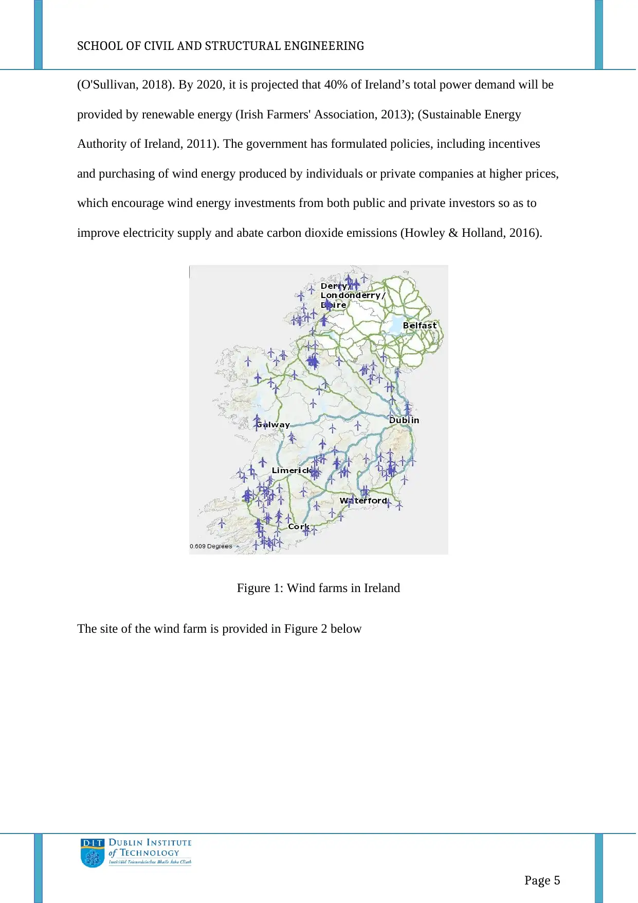
Figure 1 below shows existing wind farms in Ireland. This is mainly because the country has
very large wind resource and many parts have average wind speeds. In 2016, wind energy
accounted for 85% of renewable electricity in Ireland and 20.9% of the country’s total power
demand (Sustainable Energy Authority of Ireland , 2017). In 2017, the percentage of total
electricity demand accounted for by wind energy rose to 24% and the highest percentage
increase in installation of wind energy capacity was also recorded in the same year
Document Page
SCHOOL OF CIVIL AND STRUCTURAL ENGINEERING
Page 5
(O'Sullivan, 2018). By 2020, it is projected that 40% of Ireland’s total power demand will be
provided by renewable energy (Irish Farmers' Association, 2013); (Sustainable Energy
Authority of Ireland, 2011). The government has formulated policies, including incentives
and purchasing of wind energy produced by individuals or private companies at higher prices,
which encourage wind energy investments from both public and private investors so as to
improve electricity supply and abate carbon dioxide emissions (Howley & Holland, 2016).
Figure 1: Wind farms in Ireland
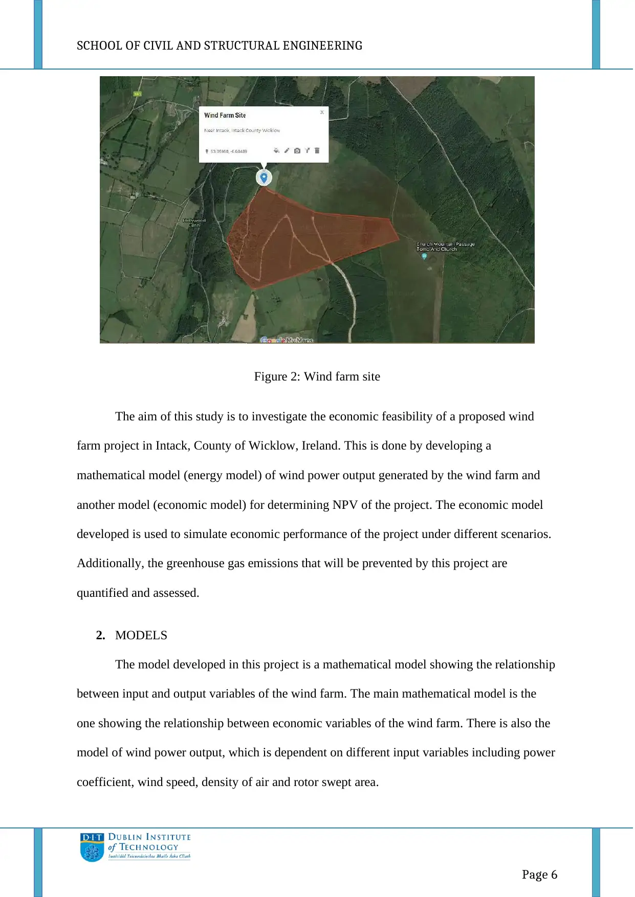
The site of the wind farm is provided in Figure 2 below
Document Page
SCHOOL OF CIVIL AND STRUCTURAL ENGINEERING
Page 6
Figure 2: Wind farm site
The aim of this study is to investigate the economic feasibility of a proposed wind
farm project in Intack, County of Wicklow, Ireland. This is done by developing a
mathematical model (energy model) of wind power output generated by the wind farm and
another model (economic model) for determining NPV of the project. The economic model
developed is used to simulate economic performance of the project under different scenarios.
Additionally, the greenhouse gas emissions that will be prevented by this project are
quantified and assessed.
2. MODELS
The model developed in this project is a mathematical model showing the relationship
between input and output variables of the wind farm. The main mathematical model is the
one showing the relationship between economic variables of the wind farm. There is also the
model of wind power output, which is dependent on different input variables including power
coefficient, wind speed, density of air and rotor swept area.

Paraphrase This Document

Need a fresh take? Get an instant paraphrase of this document with our AI Paraphraser
Document Page
SCHOOL OF CIVIL AND STRUCTURAL ENGINEERING
Page 7
2.1. Flow model diagram
Figure 3 below is the flow model diagram of the wind farm. The wind turbines convert
kinetic energy from the wind into mechanical or rotational energy. The coupling and gear
system steps up the speed of the mechanical energy and transfers to the rotor of the generator.
The generator converts mechanical energy and electrical energy (electricity). The controller
detects the wind speed, wind direction, temperature and output from the generator then
initiates appropriate signals to control them. The transformer manipulates power voltage level
for safe transmission. The substation increases or reduces voltage before the electricity is
connected to the power grid. The power grid distributes the electricity to the final consumers.
Figure 3: Flow model diagram
2.2. Wind Power Output model
Intack, County of Wicklow is one of the regions with average wind speeds in Ireland. The
average windiest, windier and calmer months of the year in Wicklow records average wind
speeds of 18.1 mph (8.09 m/s), 14.5 mph (6.48 m/s) and 10.8 mph (4.83 m/s) respectively
(Weather Spark, 2018). It is important to note that these wind speeds are the average of the
entire Wicklow region. The wind speeds vary from one season to another. Considering that
the onshore site where the wind farm in this project is planned to be constructed is along the
coastline bordering the Irish Sea, the wind speed in the region is definitely higher than the
Wind Wind
turbines
Coupling and gear
system Generator Transformer
SubstationPower grid
Controller
Consumers
Document Page
SCHOOL OF CIVIL AND STRUCTURAL ENGINEERING
Page 8
average calmer, windier and windiest values. Therefore the wind power output in this project
is calculated using average wind speed of 18.5 mph (8.26 m/s). This value is obtained from
the IEA Wind website (IEA Wind, (n.d.)).
The amount of power output that a turbine can generate is calculated using equation 1 below
(Rozenblat, 2012)
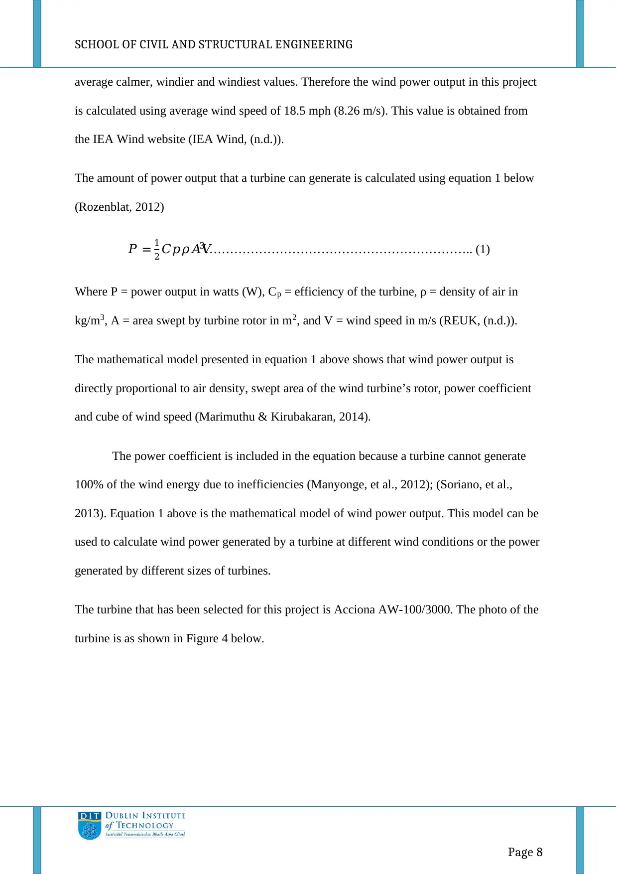
𝑃 = 1
2 𝐶𝑝𝜌𝐴𝑉3……………………………………………………….. (1)
Where P = power output in watts (W), Cp = efficiency of the turbine, ρ = density of air in
kg/m3, A = area swept by turbine rotor in m2, and V = wind speed in m/s (REUK, (n.d.)).
The mathematical model presented in equation 1 above shows that wind power output is
directly proportional to air density, swept area of the wind turbine’s rotor, power coefficient
and cube of wind speed (Marimuthu & Kirubakaran, 2014).
The power coefficient is included in the equation because a turbine cannot generate
100% of the wind energy due to inefficiencies (Manyonge, et al., 2012); (Soriano, et al.,
2013). Equation 1 above is the mathematical model of wind power output. This model can be
used to calculate wind power generated by a turbine at different wind conditions or the power
generated by different sizes of turbines.
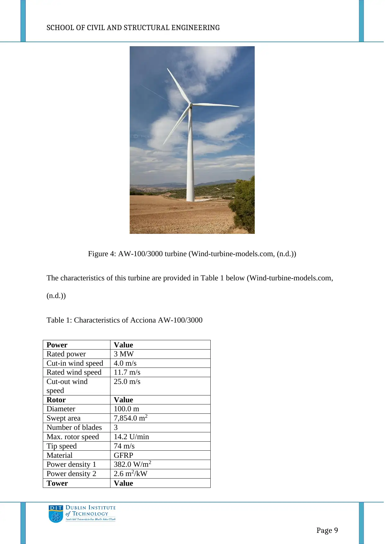
The turbine that has been selected for this project is Acciona AW-100/3000. The photo of the
turbine is as shown in Figure 4 below.
Document Page
SCHOOL OF CIVIL AND STRUCTURAL ENGINEERING
Page 9
Figure 4: AW-100/3000 turbine (Wind-turbine-models.com, (n.d.))
The characteristics of this turbine are provided in Table 1 below (Wind-turbine-models.com,
(n.d.))
Table 1: Characteristics of Acciona AW-100/3000
Power Value
Rated power 3 MW
Cut-in wind speed 4.0 m/s
Rated wind speed 11.7 m/s
Cut-out wind
speed
25.0 m/s
Rotor Value
Diameter 100.0 m
Swept area 7,854.0 m2
Number of blades 3
Max. rotor speed 14.2 U/min
Tip speed 74 m/s
Material GFRP
Power density 1 382.0 W/m2
Power density 2 2.6 m2/kW
Tower Value

Secure Best Marks with AI Grader

Need help grading? Try our AI Grader for instant feedback on your assignments.
Document Page
SCHOOL OF CIVIL AND STRUCTURAL ENGINEERING
Page 10
Rotor swept area, A = πr2 = π x 502 = 7,854 m2
Density of air, ρ = 1.25 kg/m3
Velocity, v = 8.26 m/s
Power coefficient, Cp = it usually ranges from 25% to 45% hence the chosen value is 35% =
0.35
𝑃 = 1
2 𝐶𝑝𝜌𝐴𝑉3 = 1
2 𝑥 0.35 𝑥 1.25 𝑥 7854 𝑥 8.263 = 𝟎. 𝟗𝟕 𝑴𝑾
The mathematical model provided in Equation 1 above is used to simulate wind
power output from the wind turbine at different wind speeds. This is so as to determine the
effect of wind fluctuation on wind power generated. The model also helps in determining the
minimum wind power output that the turbine can produce at cut-in wind speed, rated wind
speed and cut-out wind speed. Generally, the turbine cannot produce power exceeding the
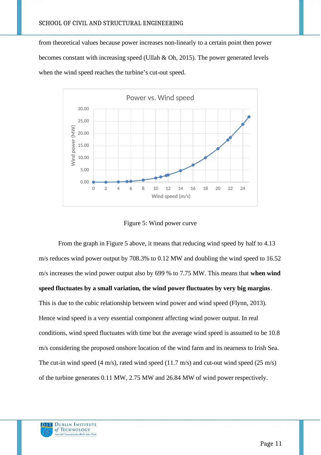
one generated at cut-out wind speed. Figure 5 below shows the relationship between wind
power output and wind speed of the turbine when all other parameters (power coefficient,
diameter of the turbine and density of air) remain constant. This graph has been drawn
through simulation of the mathematical model provided in Equation 1 using different wind
speeds. The graph in Figure 5 below is similar to a typical power-wind speed graph drawn
Type Concrete
Shape Conical
Hub height 100/120 m
Corrosion
protection
Painted
Weight Value
Rotor 66.0 tonnes
Hub 32.0 tonnes
Nacelle 118.0 tonnes
Max. tower 1,100.0 tonnes
Total weight 1,284.0 tonnes
Manufacturer Acciona Energy S.A. from
Spain
Document Page
SCHOOL OF CIVIL AND STRUCTURAL ENGINEERING
Page 11
from theoretical values because power increases non-linearly to a certain point then power
becomes constant with increasing speed (Ullah & Oh, 2015). The power generated levels
when the wind speed reaches the turbine’s cut-out speed.
Figure 5: Wind power curve
From the graph in Figure 5 above, it means that reducing wind speed by half to 4.13
m/s reduces wind power output by 708.3% to 0.12 MW and doubling the wind speed to 16.52
m/s increases the wind power output also by 699 % to 7.75 MW. This means that when wind
speed fluctuates by a small variation, the wind power fluctuates by very big margins.
This is due to the cubic relationship between wind power and wind speed (Flynn, 2013).
Hence wind speed is a very essential component affecting wind power output. In real
conditions, wind speed fluctuates with time but the average wind speed is assumed to be 10.8
m/s considering the proposed onshore location of the wind farm and its nearness to Irish Sea.
The cut-in wind speed (4 m/s), rated wind speed (11.7 m/s) and cut-out wind speed (25 m/s)
of the turbine generates 0.11 MW, 2.75 MW and 26.84 MW of wind power respectively.
0.00
5.00
10.00
15.00
20.00
25.00
30.00
0 2 4 6 8 10 12 14 16 18 20 22 24
Wind power (MW)
Wind speed (m/s)
Power vs. Wind speed
Document Page
SCHOOL OF CIVIL AND STRUCTURAL ENGINEERING
Page 12
The wind farm in this project will comprise of 10 turbines. Hence the total wind power
generated at a time is calculated as follows:
0.97W x 10 = 9.7 MW
Hence the overall mathematic model of wind power output generated by the wind farm
comprising of 10 turbines is given as:
𝑃 = 1
2 𝐶𝑝𝜌𝐴𝑉3𝑥 10 = 5𝐶𝑝𝜌𝐴𝑉3 = 5 𝑥 0.35 𝑥 1.25 𝑥 7854 𝑥 8.263 = 𝟗. 𝟕 𝑴𝑾
An average turbine has a lifespan ranging between 20 and 25 years (Jacobson, 2016).
However, studies have shown that wind turbines are wearing and tearing faster than projected
thus their capacity declines faster (Mendick, 2012). When the output of the turbines
decreases, the levelized cost of electricity (LCOE) of the wind farm increases. It is estimated
that the output of onshore wind farms reduces by 16% in ten years mainly due to wear and
tear (Staffell & Green, 2014). The lifespan of this project is 20 years, using a typical service
life of modern turbines (Ziegler, et al., 2018).
2.3. Economic model
The economic feasibility of this project is evaluated using net present value (NPV).
The NPV is determined on the principle that risks are inevitable in renewable energy projects
hence it is important to discount the capital cost of the project so as to estimate the real or
actual future costs and benefits of the project (Zizlavsky, 2014). The NPV determines the
difference between discounted cash outflows and discounted cash inflows. A positive NPV
value shows that the project will generate profit hence there will be value added to the
project. On the other hand, a negative NPV shows that the project will incur losses hence no
value will be added to the project (Gaspars-Wieloch, 2017). Therefore the higher the NPV the
better the project.

Paraphrase This Document

Need a fresh take? Get an instant paraphrase of this document with our AI Paraphraser
Document Page
SCHOOL OF CIVIL AND STRUCTURAL ENGINEERING
Page 13
The general equation of determining NPV is provided in equation 2 below
𝑁𝑃𝑉 = 𝐹𝑛
(1+𝑑)𝑛 = 𝐹0
(1+𝑑)0 + 𝐹1
(1+𝑑)1 + 𝐹2
(1+𝑑)2 + ⋯ + 𝐹𝑁
(1+𝑑)𝑁
𝑁
𝑛=0 ………………………. (2)
Where Fn = net cash flow generated in year n, d = annual discount rate and N = period of
analysis in years. The individual terms in equation 2 above is the present value meaning that
PV is obtained by adding the present values of the project period.
Economic analysis of the wind farm entails determining the investment cost, operations and
maintenance costs, and the total revenue from the electricity generated, and in consideration
of other elements such as internal rate of investment (IRR), discounted rate (r), and lifespan
of the wind farm.
2.3.1. Investment cost
The cost of wind farms is influenced by a broad range of factors including, but not
limited to: location of the wind farm, number and size of turbines, power coefficient, wind
resource in the region, and government policies (including subsidies, incentives, taxes and
permits), among others (De Olveira, 2012). The investment costs in this project comprise of
land rent, turbines, consultancy, foundation, road construction, consultancy, grid connection,
electric installation and control systems. Turbine cost accounts for the biggest share of the
total investment cost, usually over 75%.
Total investment cost (this is the initial investment or capital cost including cost of
turbines and other materials and construction/installation cost) of the wind farm is calculated
as follows:
Total investment cost = investment cost per kW of wind energy x wind energy output of the
wind farm
Document Page
SCHOOL OF CIVIL AND STRUCTURAL ENGINEERING
Page 14
The average investment cost per kW of wind energy in Ireland is obtained from IEA Wind
website. This value is €1,677 per kW for the year 2016 (IEA Wind, (n.d.)).
Total investment costs = €1,677 per kW x 9.7 x 10³ kW = €16,266,900
In most cases, investment cost is usually a one-time expenditure but in this project, it
is assumed that the wind farm will be constantly improved throughout the project period.
Therefore the investment cost is assumed to be 5% of the original capital or investment cost.
This means that the annual investment cost of the project from the 1st to the 20th year will be:
5
100 𝑥 €16,266,900 = €𝟖𝟏𝟑, 𝟎𝟑𝟒𝟓
The annual investment cost will be used to buy new components and other necessary
improvements and for miscellaneous expenses to ensure that the turbines maintain their
power coefficient throughout the period.
2.3.2. Operations and maintenance (O&M) costs
O&M costs account for a significant percentage of a wind turbine’s total annual costs.
These costs usually make about 20-25% of the total annual investment costs (Morthorst, et
al., 2012). The O&M costs include costs incurred in regular repair and maintenance of the
wind farm, insurance, purchase of spare parts and administration costs, among others.
The O&M costs of the wind farm in a year is obtained as follows:
Total O&M costs = annual O&M costs per kW x total kW
The average annual O&M costs of a wind farm in Ireland is €34 per kW.
Total O&M costs = €34 per kW x 9.7 x 10³ kW = €329,800
Document Page
SCHOOL OF CIVIL AND STRUCTURAL ENGINEERING
Page 15
2.3.3. Revenue generated
The annual revenue generated from the wind farm is calculated as follows:
Revenue = price of electricity per kWh x annual kWh produced
The turbines are estimated to operate optimally for 20 hours a day throughout the year at the
average wind speed. Therefore the amount of electricity that the wind farm will generate per
year is calculated as follows:
= 9.7 MW x 20 hours per day x 365 days = 70,810 MWh = 70,810 x 103 kWh
The average price of electricity in Ireland is €0.18 per kWh. This is inclusive of all applicable
taxes, levies and standing charges.
Therefore annual revenue = €0.18 per kWh x 70,810 x 103 kWh = €12,745,800
It is assumed that the wind turbines will operate optimally throughout the 20-year period and
therefore revenues generated will remain constant during the lifespan of the project. The
projected is expected to have a straight-line deprecation over a period of 15 years. The
discount rate is 10%. The wind farm will also attract a corporation tax rate of 15% throughout
its lifespan. The projected annual inflation rate over the 20-year period is 2%. The weighted
average cost of capital (WACC) is taken to be 12%.
𝐷𝑒𝑝𝑟𝑒𝑐𝑖𝑎𝑡𝑖𝑜𝑛 =
𝐷𝑒𝑝𝑟𝑒𝑐𝑖𝑎𝑡𝑖𝑜𝑛 𝑟𝑎𝑡𝑒
100 𝑥 𝐼𝑛𝑣𝑒𝑠𝑡𝑚𝑒𝑛𝑡 𝑐𝑜𝑠𝑡
Net taxable income = revenue – O&M costs – depreciation
𝐶𝑜𝑟𝑝𝑜𝑟𝑎𝑡𝑒 𝑡𝑎𝑥 =
𝐶𝑜𝑟𝑝𝑜𝑟𝑎𝑡𝑖𝑜𝑛 𝑡𝑎𝑥 𝑟𝑎𝑡𝑒
100 𝑥 𝑁𝑒𝑡 𝑡𝑎𝑥𝑎𝑏𝑙𝑒 𝑖𝑛𝑐𝑜𝑚𝑒
After tax cash flow = revenue – O&M costs – investment costs – corporation tax
The NPV is calculated using real discount rate. The real discount rate is calculated as follows:

Secure Best Marks with AI Grader

Need help grading? Try our AI Grader for instant feedback on your assignments.
Document Page
SCHOOL OF CIVIL AND STRUCTURAL ENGINEERING
Page 16
(1 + dn) = (1 + dr)(1 + e); where dn = nominal discount rate, dr = real discount rate and e =
inflation rate
Rearranging the above equation gives
𝑑𝑟 = (1+𝑑𝑛)
(1+𝑒) 1; but dn = 12% = 0.12 and e = 2% = 0.02
Therefore 𝑑𝑟 = (1+0.12)
(1+0.02) 1 = 0.098 = 9.8%
The dr is then used to calculate the discount factor for each year as follows:
𝐷𝑖𝑠𝑐𝑜𝑢𝑛𝑡 𝑓𝑎𝑐𝑡𝑜𝑟 =
1
(1+𝑑𝑟)𝑛 ; where n is the number of year
The discount factors for the 20 years are as shown in Table 2 below
Table 2: Discount factors of the project
Year Discount factor
0 1.000
1 0.911
2 0.829
3 0.755
4 0.688
5 0.627
6 0.571
7 0.520
8 0.473
9 0.431
10 0.393
11 0.358
12 0.326
13 0.297
14 0.270
15 0.246
16 0.224
17 0.204
18 0.186
19 0.169
20 0.154
Document Page
SCHOOL OF CIVIL AND STRUCTURAL ENGINEERING
Page 17
3. ECONOMIC MEASURES
This projects has been evaluated using three economic measures discussed below
3.1. Net Present value (NPV)
One of the economic measures used to assess this project is the NPV. The NPV is simply
the sum of the present values throughout the project lifespan. The present values have been
calculated using equation 2 above i.e. multiplying the after tax cash flow with the discount
factor. The NPV is the determined by adding the present values throughout the project
lifespan. From the calculations in Excel, the NPV of the wind farm is €69,679,384.
NPV is been selected to be used for analyzing the economic feasibility of this project
instead of using internal rate of investment (IRR) because the former is more reliable than the
latter. IRR is not appropriate for this project because it is applicable where NPV = 0 (Arshad,
2012). NPV is an appropriate economic measure because it estimates the current value of the
project by taking into account several factors that will affect the value of the project in the
future, including the discount rate, corporation tax rate, inflation rate, depreciation rate and
other inherent risks (Borad, 2018); (Keythman, 2018). NPV also determines whether the
investment made in the project will create value and estimates the value in Euros (€).
There are several assumptions that have been made when calculating the NPV for the project.
Some of the assumptions include:
The annual investment cost will be the same throughout the project lifespan from the
1st to the 20th year.
The wind power output generated from the wind farm will remain constant during the
entire project period.
The price of electricity per kWh will remain the same throughout the project period.
O&M costs of the project will be constant during the 20-year project lifespan.
Document Page
SCHOOL OF CIVIL AND STRUCTURAL ENGINEERING
Page 18
The corporation tax, discount and inflation rate will remain unchanged during the
project lifespan.
Depreciation rate will remain the same throughout the 15 year period when the
depreciation will be applicable.
Annual revenue generated from the project will be the same throughout the project
lifespan.
Therefore the general mathematical model of calculating NPV for the wind farm project is
provided in equation 3 below
𝑁𝑃𝑉 = 𝐹𝑛
(1+𝑑𝑟)𝑛 = 𝐹0
(1+𝑑𝑟)0 + 𝐹1
(1+𝑑𝑟)1 + 𝐹2
(1+𝑑𝑟)2 + ⋯ + 𝐹20
(1+𝑑𝑟)20
𝑁
𝑛=0 ……………………. (3)
Where Fn = net cash flow generated in nth year, d = real annual discount rate and N =
lifespan of the project in years.
Fn = Rn OMn In Tn
Where Rn = revenue generated for the nth year, OMn = operations and maintenance costs
incurred during the nth year, In = investment costs incurred in the nth year, and Tn =
corporation tax paid in the nth year.
The summary of investment costs, O&M costs, revenues, depreciation, net taxable income,
corporation tax, net cash flows, and present values and NPV is provided in Appendix 1.
3.2. Payback period
Payback period is a method that is used to estimate the amount of time that a project’s
cash flows will take to repay the project’s initial investment cost (AccountingTools, 2018).
The main reason why payback period has been selected as an economic measure is because it
is a very simple method and provides quick evaluation. This method is most appropriate for

Paraphrase This Document

Need a fresh take? Get an instant paraphrase of this document with our AI Paraphraser
Document Page
SCHOOL OF CIVIL AND STRUCTURAL ENGINEERING
Page 19
projects with consistent cash flows, which is the case for the project in this paper. Lastly, this
method is also very appropriate in industries that are experiencing rapid technological
changes with increase uncertainty (Borad, 2017).
Payback period is a very essential parameter of estimating the time it will take for the
project to recover the invest costs incurred in the project. A project with a shorter payback
period is more attractive than the one with a longer payback period.
The payback period of the project can be calculated as follows (Accounting Explained,
2013):
𝐷𝑖𝑠𝑐𝑜𝑢𝑛𝑡𝑒𝑑 𝑝𝑎𝑦𝑏𝑎𝑐𝑘 𝑝𝑒𝑟𝑖𝑜𝑑 = 𝑃 +
𝑄
𝑅
Where P is the last period with a –ve (negative) discounted present value; Q is the absolute
value of the discounted cumulative present value of period P; and R is the discounted present
value of the subsequent period after period P.
𝐷𝑖𝑠𝑐𝑜𝑢𝑛𝑡𝑒𝑑 𝑝𝑎𝑦𝑏𝑎𝑐𝑘 𝑝𝑒𝑟𝑖𝑜𝑑 = 1 +
|7173768|
8281540.6= 1 + 0.86623 ≈ 1.9 𝑦𝑒𝑎𝑟𝑠
This means that the investment cost of the project will be recovered after 1.9 years if the
wind farm operates as expected in this project. This is a very short repayment period and
therefore the project should be implemented as planned. The payment period also supports
the big NPV calculated above hence this project is economically viable.
3.3. Cost benefit ratio (CBR)
This is another economic measure used in the project because it shows the relationship
between the expenses (costs) and gains (benefits) of the project. The main advantages of
CBR are: it provides adequate clarity about the project diving into the project’s specifics;
assesses the overall feasibility of the project; considers the current affordability of the project;
Document Page
SCHOOL OF CIVIL AND STRUCTURAL ENGINEERING
Page 20
can help make accurate predictions about the project’s economic performance; and can help
in establishing useful policies applicable to the project (Gaille, 2018).
This project will have numerous economic, environmental and social impacts and
therefore it is necessary to determine its CBR. The CBR is very essential especially when
considering the long-term social and financial sustainability of the project (Maravas &
Pantouvakis, 2018).
The CBR of the project is calculated as follows:
𝐶𝐵𝑅 =
𝑃𝑉 𝑜𝑓 𝑎𝑙𝑙 𝑏𝑒𝑛𝑒𝑓𝑖𝑡𝑠 (𝐹𝑛)
𝑃𝑉 𝑜𝑓 𝑎𝑙𝑙 𝑐𝑜𝑠𝑡𝑠 (𝐶𝑛)
= 𝐹𝑛
(1+𝑑𝑟)𝑛
𝑁
𝑛=0
𝐶𝑛
(1+𝑑𝑟)𝑛
𝑁
𝑛=0
;
From the values in Excel, the CBR is
𝐶𝐵𝑅 =
69679384
26133484= 2.666 ≈ 2.7
Since the CBR is greater than one, it means that the project will have a positive NPV (which
is the case as per the above calculations) and that the internal rate of investment (IRR) will be
greater than the discount rate.
4. SENSITIVITY ANALYSIS
This process involves varying different parameters affecting the cost and revenues of the
project independently so as to establish the performance of the project under different
scenarios. It also helps in determining a logical situation in the future.
4.1. Scenario 1
Scenario 1 is higher electricity price and lower corporation tax rate
When electricity price is increased from €0.18 to €0.24, the total annual revenue becomes:
Document Page
SCHOOL OF CIVIL AND STRUCTURAL ENGINEERING
Page 21
= €0.24 per kWh x 70,810 x 103 kWh = €16,994,400
The corporation tax rate is also reduced from 15% to 10%
𝐷𝑖𝑠𝑐𝑜𝑢𝑛𝑡𝑒𝑑 𝑝𝑎𝑦𝑏𝑎𝑐𝑘 𝑝𝑒𝑟𝑖𝑜𝑑 = 1 +
|3199992.896|
11900643.99= 1 + 0.2689 ≈ 1.3 𝑦𝑒𝑎𝑟𝑠
𝐶𝐵𝑅 =
107414833.2
26133484 = 4.111 ≈ 4.1
Detailed calculations of this scenario is provided in Appendix 2 and the excel spreadsheet.
The comparison of NPV, payback period and CBR of the original scenario and scenario 1 is
provided in Table 3 below
Table 3: Economic measures of scenario 1
Original scenario Scenario 1
Electricity price per kWh 0.18 0.24
Corporation tax rate 15% 10%
NPV 69,679,384 107,414,833.2
Payback period 1.9 years 1.3 years
CBR 2.7 4.1
An increase in price of electricity per kWh and a decrease in corporation tax rate will
significantly increase both the NPV and CBR of the project, and decrease the payback period.
This means that the investment cost will be repaid faster and the value of the net project of
the project at the end of its lifespan will be higher than the original scenario.
4.2. Scenario 2
Scenario 2 is lower electricity price and higher inflation rate
When electricity price decreases from the current €0.18 to €0.12, the total annual revenue
becomes:
= €0.12 per kWh x 70,810 x 103 kWh = €8,497,200

Secure Best Marks with AI Grader

Need help grading? Try our AI Grader for instant feedback on your assignments.
Document Page
SCHOOL OF CIVIL AND STRUCTURAL ENGINEERING
Page 22
The inflation rate is also increased from 2% to 5%. This changes the real discount rate (dr)
and the discount factor
WACC or dn = 12% = 0.12
Inflation, e = 5% = 0.05
Hence 𝑑𝑟 = (1+0.12)
(1+0.05) 1 = 0.0667 = 6.7%
𝐷𝑖𝑠𝑐𝑜𝑢𝑛𝑡𝑒𝑑 𝑝𝑎𝑦𝑏𝑎𝑐𝑘 𝑝𝑒𝑟𝑖𝑜𝑑 = 2 +
|4696402.13|
5256228 = 2 + 0.893 ≈ 2.9 𝑦𝑒𝑎𝑟𝑠
𝐶𝐵𝑅 =
52470234
28664985= 1.83 ≈ 4.1
Detailed calculations of this scenario is provided in Appendix 3 and the excel spreadsheet.
The comparison of NPV, payback period and CBR of the original scenario and scenario 2 is
provided in Table 4 below
Table 4: Economic measures of scenario 2
Original scenario Scenario 2
Electricity price per kWh 0.18 0.12
Inflation rate 2% 5%
NPV 69,679,384 52,470,234
Payback period 1.9 years 2.9 years
CBR 2.7 1.8
When the price of electricity per kWh is decreased and the inflation rate increased, the
NPV and CBR of the project will decrease while the payback period will increase. This
implies that it will take longer to repay the initial investment cost of the project and the net
value of the project at the end of its lifespan will be less compared with the original scenario
of the project.
4.3. Scenario 3
Scenario 3 is lower investment and O&M costs and lower depreciation rate
Document Page
SCHOOL OF CIVIL AND STRUCTURAL ENGINEERING
Page 23
Total investment costs = €1,200 per kW x 9.7 x 10³ kW = €11,640,000
The investment cost was assumed to be 5% of the original capital or investment cost.
Therefore the annual investment cost of the project from the 1st to the 20th year becomes:
5
100 𝑥 €11,640,000 = €582,000
The total O&M costs = €25 per kW x 9.7 x 10³ kW = €242,500
The depreciation rate also decreases from 10% to 5% over a period of 15 years (straight-line
depreciation).
𝐷𝑖𝑠𝑐𝑜𝑢𝑛𝑡𝑒𝑑 𝑝𝑎𝑦𝑏𝑎𝑐𝑘 𝑝𝑒𝑟𝑖𝑜𝑑 = 1 +
|2411306.922|
8405003 = 1 + 0.287 ≈ 1.3 𝑦𝑒𝑎𝑟𝑠
𝐶𝐵𝑅 =
75737882
18756332= 4.03 ≈ 4.0
Detailed calculations of this scenario is provided in Appendix 4 and the excel spreadsheet.
The comparison of NPV, payback period and CBR of the original scenario and scenario 3 is
provided in Table 5 below
Table 5: Economic measures of scenario 3
Original scenario Scenario 3
Investment cost per kW 1,677 1,200
O&M costs per kW 34 25
Depreciation rate 10% 5%
NPV 69,679,384 75,737,882
Payback period 1.9 years 1.3 years
CBR 2.7 4.0
Reducing the investment and O&M costs and decreasing the depreciation rate (or
WACC) will result to an increase in NPV and CBR and a decrease in repayment period. This
means that it will take less time to recover the initial investment cost of the project and the
Document Page
SCHOOL OF CIVIL AND STRUCTURAL ENGINEERING
Page 24
net value of the project at the end of the project’s lifespan will be greater than that of the
original scenario.
4.4. Scenario 4
Scenario 4 is higher weighted average cost of capital (WACC) and higher inflation rate
A change in WACC and inflation rate results to a change in real discount and discount
factors. Hence the real discount becomes
𝑑𝑟 = (1+𝑑𝑛)
(1+𝑒) 1; Where dn = 20% = 0.2 and e = 5% = 0.05
Therefore 𝑑𝑟 = (1+0.2)
(1+0.05) 1 = 0.1429 = 14.3%
The dr is then used to calculate the discount factor for each year as follows:
𝐷𝑖𝑠𝑐𝑜𝑢𝑛𝑡 𝑓𝑎𝑐𝑡𝑜𝑟 =
1
(1+𝑑𝑟)𝑛 ; Where n is the number of year
𝐷𝑖𝑠𝑐𝑜𝑢𝑛𝑡𝑒𝑑 𝑝𝑎𝑦𝑏𝑎𝑐𝑘 𝑝𝑒𝑟𝑖𝑜𝑑 = 1 +
|7531765.704
7642287 = 1 + 0.986 ≈ 2.0 𝑦𝑒𝑎𝑟𝑠
𝐶𝐵𝑅 =
48620988
23709046= 2.05 ≈ 2.1
Detailed calculations of this scenario is provided in Appendix 5 and the excel spreadsheet.
The comparison of NPV, payback period and CBR of the original scenario and scenario 4 is
provided in Table 6 below
Table 6: Economic measures of scenario 4
Original scenario Scenario 4
WACC/discount rate 12% 20%
Inflation rate 2% 5%
NPV 69,679,384 48,620,988
Payback period 1.9 years 2.0 years
CBR 2.7 2.1

Paraphrase This Document

Need a fresh take? Get an instant paraphrase of this document with our AI Paraphraser
Document Page
SCHOOL OF CIVIL AND STRUCTURAL ENGINEERING
Page 25
When the WACC/discount rate is decreased and the inflation rate increased, there will be
a decrease in NPV and CBR of the project. However, the payback period of the project will
increase. This implies that the time taken to recover the initial investment cost will be longer
and the net value of the project at the end of the project lifespan will be less compared to that
of the original scenario.
4.5. Scenario 5
Scenario 5 is higher wind speed, lower O&M costs, and higher electricity price
An increase in wind speed will result to an increase in wind power output and all the other
parameters proportional to it such as investment and O&M costs. The wind speed is increased
from 8.26 m/s to 12 m/s hence the power output becomes
𝑃 = 1
2 𝐶𝑝𝜌𝐴𝑉3𝑥 10 = 5𝐶𝑝𝜌𝐴𝑉3 = 5 𝑥 0.35 𝑥 1.25 𝑥 7854 𝑥 123 = 29.7 𝑀𝑊
Total investment costs becomes = €1,677 per kW x 29.7 x 10³ kW = €49,806,900
The O&M costs is also reduced from €34 per kWh to €25 per kWh
Total O&M costs becomes = €25 per kW x 29.7 x 10³ kW = €742,500
The price of electricity is also increased from €0.18 to €0.24. This means annual revenue
generated is:
= 29.7 MW x 20 hours per day x 365 days = 216,810 MWh = 216,810 x 103 kWh
Annual revenue = €0.24 per kWh x 216,810 x 103 kWh = €52,034,400
𝐷𝑖𝑠𝑐𝑜𝑢𝑛𝑡𝑒𝑑 𝑝𝑎𝑦𝑏𝑎𝑐𝑘 𝑝𝑒𝑟𝑖𝑜𝑑 = 1 +
|11687707
34716933.17
= 1 + 0.3367 ≈ 1.3 𝑦𝑒𝑎𝑟𝑠
𝐶𝐵𝑅 =
310745851.1
77709868 = 3.999 ≈ 4.0
Document Page
SCHOOL OF CIVIL AND STRUCTURAL ENGINEERING
Page 26
Detailed calculations of this scenario is provided in Appendix 6 and the excel spreadsheet.
The comparison of NPV, payback period and CBR of the original scenario and scenario 5 is
provided in Table7 below
Table 7: Economic measures of scenario 5
Original scenario Scenario 5
Wind speed 8.26 12 m/s
O&M costs 34 25
Electricity price per kWh 0.18 0.24
NPV 69,679,384 222,335,325.8
Payback period 1.9 years 1.3 years
CBR 2.7 4.0
When wind speed is increased, price of electricity per kWh is increased and O&M costs
reduced, the NPV of the project will increase significantly, CBR will also increase, and the
payback period of the project will decrease. This means that it will take shorter time to
recover the initial investment cost of the project and the net value of the project will be very
high at the end of the project’s lifespan.
5. GREENHOUSE GAS EMISSIONS
Reduced greenhouse gas emissions is one of the major advantages of wind energy. This is
because production of wind energy does not involve burning of fossil fuels like it is the case
with conventional power plants. Wind energy is generated by wind turbines that converts
kinetic energy from the moving air into mechanical energy that is then converted into
electricity by a generator. This process does not emit any greenhouse gases or air pollutants
(Lloyd, 2014). Wind energy production reduces significant amounts of carbon, nitrogen
oxides, sulfur dioxide and air pollutants that trigger asthma attacks and crate smog. In 2017,
wind energy generation avoided approximately 189 x 106 metric tonnes of carbon dioxide
emissions, 122 x 103 tonnes of nitrogen oxides and 188 x 103 tonnes of sulfur dioxide
(American Wind Energy Association, 2018). However, it is important to note that some
Document Page
SCHOOL OF CIVIL AND STRUCTURAL ENGINEERING
Page 27
phases of wind energy production lifecycle produces emissions. These include manufacturing
of the wind turbines, transportation of the wind turbines and installation of the wind turbines
(Rinkesh, (n.d.)). Maintenance and decommissioning of wind turbines also produce some
greenhouse gas emissions but they are very minimal compared with other energy sources. A
typical wind farm repays the carbon footprint produced in these phases within six months of
operation and avoids carbon emissions throughout its lifespan. Figure 6 below shows
estimated carbon dioxide emissions avoided by wind energy production over the years.
Figure 6: Carbon dioxide emissions avoided by wind energy (American Wind Energy
Association, 2018)
In this paper, the amount of greenhouse gas emissions that will be avoided by the
project is determined by comparing the amount of carbon emissions that the wind farm in this
project will produce and the one that a typical coal plant would produce over the same
lifespan.

Secure Best Marks with AI Grader

Need help grading? Try our AI Grader for instant feedback on your assignments.
Document Page
SCHOOL OF CIVIL AND STRUCTURAL ENGINEERING
Page 28
A typical coal power plant produces approximately 900 g of CO2 equivalent (CO2e)/kWh of
electricity generated whereas a wind energy produces an estimated 11 g of CO 2e/kWh of
electricity generated (Schipani, 2018).
However, wind farm in this project is estimated to generate 70,810 x 103 kWh of electricity
each year. This means that at the end of its 20-year lifespan, the wind farm will have
generated
70,810 x 103 kWh/year x 20 years = 1416.2 x 106 kWh
Carbon emissions from the wind farm
1 kWh = 11 g of CO2e
1416.2 x 106 kWh = 1416.2 𝑥 106𝑘𝑊ℎ 𝑥 11 𝑔 𝑜𝑓 𝐶𝑂2𝑒
1 𝑘𝑊ℎ = 15578.2 𝑥 106𝑔 𝑜𝑓 𝐶𝑂2𝑒
1 x 10⁶ g = 1 tonne
15578.2 x 106 g = = 15578.2 𝑥 106 𝑔 𝑥 1 𝑡𝑜𝑛𝑛𝑒
1 𝑥 106𝑔 = 15,578.2 𝑡𝑜𝑛𝑛𝑒𝑠 𝑜𝑓 𝐶𝑂2𝑒
Carbon emissions from an equivalent coal plant
1 kWh = 900 g of CO2e
1416.2 x 106 kWh = 1416.2 𝑥 106𝑘𝑊ℎ 𝑥 900 𝑔 𝑜𝑓 𝐶𝑂2𝑒
1 𝑘𝑊ℎ = 1274580 𝑥 106𝑔 𝑜𝑓 𝐶𝑂2𝑒
1 x 10⁶ g = 1 tonne
1274580 x 106 g = = 1274580 𝑥 106 𝑔 𝑥 1 𝑡𝑜𝑛𝑛𝑒
1 𝑥 106𝑔 = 1,274,580 𝑡𝑜𝑛𝑛𝑒𝑠 𝑜𝑓 𝐶𝑂2𝑒
This means that during the 20-year period, the amount of carbon emissions that will have
been avoided by the wind farm is
Document Page
SCHOOL OF CIVIL AND STRUCTURAL ENGINEERING
Page 29
1,274,580 tonnes of CO2e – 15,578.2 tonnes of CO2e = 1,259,001.8 tonnes of CO2e
On annual basis, the wind energy project will avoid 62,950.09 tonnes of CO2e.
6. SITE CONSTRAINTS
There are several site constraints to the performance of wind turbines and the wind power
output produced. Some of these factors are discussed below
6.1. Spacing
Large wind turbines such as the one used in this project require extensive land area for
them to perform optimally. The 100 m rotor diameter wind turbines used in this project
require a minimum spacing of 700 between them (7 rotor diameter is the minimum spacing
required between wind turbines). Assuming that the turbines are located 700 m from each
other in two parallel lines (5 turbines in each line since the wind farm has a total of 10
turbines) that are 700 m apart with an allowance of 350 m at the edges of the perimeter of the
area. This means that the turbines alone will require a minimum space of 4.9 km2 (3.5 km by
1.4 km). Therefore it means that there must be sufficient space for the project to be
implemented is planned. This means a substantial amount of money will be spent on land
rent, depending on the location of the project. The land rent will definitely be lower if the
project is located in remote areas where land rates are low. However, the problem with
developing wind farms in remote areas is that electricity demand in these areas is low hence
there will be need to incur more costs in connecting the system to the national grid so as to
supply it to where energy demand is high. This basically implies that each choice has its
advantages and disadvantages, and comprehensive economic analysis is required before
making the final decision. It is also worth noting that the area between the wind turbines can
be put into other uses such as farming.
Document Page
SCHOOL OF CIVIL AND STRUCTURAL ENGINEERING
Page 30
6.2. Topography
Wind turbines perform well when installed in a relatively flat area with uninterrupted air
flow. Reduction of air flow interference increases wind speed and wind power output. Areas
characterized by hills or mountains and valleys are not suitable for wind turbines because
they hinder flow of wind thus decreasing wind speed. The cubic relationship between wind
power output and wind speed means that any slight reduction in wind speed will result to a
big decrease in wind power output. Installing wind turbines at higher places such as on top of
hills also improves their performance because of minimal obstruction at such heights.
6.3. Accessibility
Access to the site is another very important factor in implementation of wind farm
projects. The site should be easily accessible so as to facilitate transportation of turbines,
plant/equipment, materials, personnel and other components to and from the site. If there are
no adequate access roads, the developer must construct either temporary or permanent roads
depending on the project’s lifespan, goals and objectives. If existing roads are narrow, they
may need to be widened.
6.4. Surrounding features
This is also a major site constraint because it affects wind speed. As stated before, wind
turbines require considerable space to operate effectively. This space enables them to harness
enough wind and convert it into electrical energy. The performance of wind turbine declines
significantly if they are installed in areas surrounded by very tall buildings, mountains, trees,
or any other tall structures and features that will obstruct free movement of air. That is why
wind turbines usually have very long towers to raise the blades and prevent nearby structures
or features from obstructing wind flow (Bobby, 2014).

Paraphrase This Document

Need a fresh take? Get an instant paraphrase of this document with our AI Paraphraser
Document Page
SCHOOL OF CIVIL AND STRUCTURAL ENGINEERING
Page 31
6.5. Ground conditions
Large commercial wind turbines weigh millions of tonnes. The weight of a single wind
turbine used in this project is 1,284 tonnes. Considering the weight and height of these wind
turbines, they need to be installed on stable grounds. This means that the ground should be
stable enough to support the load imposed by the wind turbines (Denholm, et al., 2009). The
foundation of the wind turbines should also be strong enough and protected against
underground water penetration. Additionally, the site conditions should not hinder
performance of cranes and other plant and equipment used during installation, repair and
maintenance of the wind turbines.
6.6. Environmental factors
There are numerous environmental factors that affect performance of wind turbines and
transmission of electricity generated. Some of these include wind, precipitation, pressure,
humidity, temperature and lightning. For example, a saline atmosphere causes both dynamic
and static stresses as a result of cycling mechanical, electrical or thermal environments thus
causing failure of equipment used in wind energy generation and also components of
transmission lines. Temperature, precipitation, humidity and pressure also affects air density,
which is directly proportional to wind power output. Lightning can strike the wind turbine or
transmission lines thus necessitating unexpected replacement of some components. Therefore
it is important to conduct comprehensive analysis of the effect of these environmental factors
on the performance of wind turbines before constructing the wind farm.
6.7. Regulatory requirements
A wind farm cannot be developed on any site because of regulatory requirements,
including urban planning, zoning and land uses. There are requirements of the minimum
distance that wind turbines should be located from structures such as buildings, nuclear
Document Page
SCHOOL OF CIVIL AND STRUCTURAL ENGINEERING
Page 32
plants, electricity transmission les, etc. Wind zoning regulations are other requirements that
must be met before setting up a wind farm (Gaughan, 2018).
7. CONCLUSION
Wind is an environmentally friendly, inexpensive and sustainable source of energy with
numerous economic, environmental and social benefits. The amount of wind power generated
by a wind turbine depends on the wind speed, air density, diameter of wind turbine rotor and
performance coefficient of the wind turbine. Two mathematical models have been developed
in this project: one for calculating wind power output and another for calculating the NPV of
the project. The models have been used to evaluate different economic measures of the
project under varied scenarios. The economic measures used to evaluate the economic
feasibility of the project are NPV, payback period and CBR. These measures are very
essential in establishing the economic feasibility of the project hence helps companies and
developers to decide whether to invest in a project or not.
In the original scenario, the NPV, payback period and CBR of the project are
69,679,384, 1.9 years and 2.7 respectively. The mathematical models developed have been
used to assess these measures under different scenarios. Results obtained show that an
increase in price of electricity and a decrease in corporation tax rate will lead to an increase in
NPV and CBR and a decrease in payback period; a decrease in price of electricity and
inflation rate will result to a decrease in NPV and CBR and an increase in payback period; a
decrease in investment cost, O&M costs and depreciation rate will lead to an increase in NPV
and CBR and a decrease in payback period; an increase in discount rate and inflation rate will
result to a decrease in NPV and CBR and an increase in payback period; and an increase in
wind speed and price of electricity and a decrease in O&M costs will result to a significant
increase in NPV and CBR and a decrease in payback period of the project. The fourth
Document Page
SCHOOL OF CIVIL AND STRUCTURAL ENGINEERING
Page 33
scenario (scenario 4) of increasing the wind speed and price of electricity and reducing the
O&M costs provided the highest NPV and CBR values and the lowest repayment period. The
wind farm in this project will also help avoid 1,259,001.8 tonnes of CO2e over the 20-year
period.
There is great potential in production of wind energy and help reduce greenhouse gas
emissions, save money and ensure steady supply of electricity. There is need to use more
advanced technologies so as to improve efficiency of wind turbines and reduce investment
and O&M costs. The prevalence of wind energy is also increasing rapidly all over the world
with countries such as China, U.S., India, Germany, Spain and Denmark leading in wind
energy production. Therefore one way of improving wind farm projects is using advanced
technological tools to develop turbine models and simulate them so as to identify appropriate
strategies of improving their efficiency (Sarkar, et al., 2015). Countries should formulate
policies that promote growth of wind energy production, such as wind energy. Some of these
policies include ease of approving wind energy projects and issuing of permits, providing
assistance to connect wind farms to the national grid, etc. There is also need for increase
public participation so that more people can invest in wind farm projects.

Secure Best Marks with AI Grader

Need help grading? Try our AI Grader for instant feedback on your assignments.
Document Page
SCHOOL OF CIVIL AND STRUCTURAL ENGINEERING
Page 34
References
Accounting Explained, 2013. Discounted Payback Period. [Online]
Available at: https://accountingexplained.com/managerial/capital-budgeting/discounted-
payback-period
[Accessed 5 December 2018].
AccountingTools, 2018. Advantages of the Payback Period. [Online]
Available at: https://www.accountingtools.com/articles/advantages-of-the-payback-
period.html
[Accessed 5 December 2018].
American Wind Energy Association, 2018. Environmental Benefits. [Online]
Available at: https://www.awea.org/wind-101/benefits-of-wind/environmental-benefits
[Accessed 5 December 2018].
Arshad, A., 2012. Net Present Values is Better Than Internal Rate of Return.
Interdisciplinary Journal of Contemporary Research in Busness, 4(8), pp. 211-219.
Bobby, 2014. Factors Affecting Wind Power Output. [Online]
Available at: https://www.upsbatterycenter.com/blog/factors-affecting-wind-power-output/
[Accessed 5 December 2018].
Borad, S., 2017. Advantages and Disadvantages of Payback Period. [Online]
Available at: https://efinancemanagement.com/investment-decisions/advantages-and-
disadvantages-of-payback-period
[Accessed 5 December 2018].
Borad, S., 2018. Advantages and Disadvantages of NPV. [Online]
Available at: https://efinancemanagement.com/investment-decisions/advantages-and-
disadvantages-of-npv
[Accessed 5 December 2018].
De Olveira, W., 2012. Optimization Model for Economic Evaluation of Wind Farms - How
to Optimize a Wind Energy Project Economically and Technically. International Journal of
Energy Economics and Policy, 2(1), pp. 10-20.
Denholm, P., Hand, M., Jackson, M. & Ong, S., 2009. Land-Use Requirements of Modern
Wind Power Plants in the United States, Boulevard, Colorado: National Renewable Energy
Laboratory.
Flynn, J., 2013. Assessment of the Wind Energy Potential at Bausch Lomb Waterford.
Waterford, Ireland: Waterford Institute of Technology.
Gaille, B., 2018. 13 Benefit Cost Ratio Advantages and Disadvantages. [Online]
Available at: https://brandongaille.com/13-benefit-cost-ratio-advantages-and-disadvantages/
[Accessed 5 December 2018].
Document Page
SCHOOL OF CIVIL AND STRUCTURAL ENGINEERING
Page 35
Gaspars-Wieloch, H., 2017. Project Net Present Value estimation under uncertainty. Central
European Journal of Operations Research, Volume 1, pp. 1-19.
Gaughan, R., 2018. How Much Land Is Needed for Wind Turbines?. [Online]
Available at: https://sciencing.com/much-land-needed-wind-turbines-12304634.html
[Accessed 4 December 2018].
Howley, M. & Holland, M., 2016. Energy in Ireland 1990 - 2015, Dublin: Sustainable
Energy Authority of Ireland.
IEA Wind, (n.d.). Data Viewer. [Online]
Available at: https://community.ieawind.org/task26/dataviewer
[Accessed 4 December 2018].
Irish Farmers' Association, 2013. Harnessing Ireland's Wind Resource for Renewable Energy
Production, Dublin: Irish Farmers' Association (IFA).
Jacobson, R., 2016. Where Do Wind Turbines Go To Die?. [Online]
Available at: http://insideenergy.org/2016/09/09/where-do-wind-turbines-go-to-die/
[Accessed 4 December 2018].
Keythman, B., 2018. Advantages & Disadvantages of Net Present Value in Project Selection.
[Online]
Available at: https://yourbusiness.azcentral.com/advantages-disadvantages-net-present-value-
project-selection-12586.html
[Accessed 5 December 2018].
Krohn, S., Morthorst, P. & Awerbuch, S., 2009. The Economics of Wind Energy, Brussels:
European Wind Energy Association (EWEA).
Lloyd, D., 2014. Wind Energy: Advantages and Disadvantages. [Online]
Available at: http://large.stanford.edu/courses/2014/ph240/lloyd2/
[Accessed 5 December 2018].
Manyonge, A., Manyala, A., Onyango, F. & Shichika, J., 2012. Mathematical Modelling of
Wind Turbine in a Wind Energy Conversion System: Power Coefficient Analysis. Applied
Mathematical Sciences, 6(91), pp. 4527-4536.
Maravas, A. & Pantouvakis, J., 2018. A New Approach to Studying Net Present Value and
the Internal Rate of Return of Engineering Projects under Uncertainty with Three-
Dimensional Graphs. Advances in Civil Engineering, Volume 2018, pp. 1-9.
Marimuthu, C. & Kirubakaran, V., 2014. A critical review of factors affecting wind turbine
and solar cell system power production. International Journal of Advanced Engineering
Research and Studies, pp. 143-147.
Mendick, R., 2012. Wind farm turbines wear sooner than expected, says study. [Online]
Available at: https://www.telegraph.co.uk/news/earth/energy/windpower/9770837/Wind-
Document Page
SCHOOL OF CIVIL AND STRUCTURAL ENGINEERING
Page 36
farm-turbines-wear-sooner-than-expected-says-study.html
[Accessed 4 December 2018].
Morthorst, P., Auer, H., Garrad, A. & Blanco, I., 2012. Wind Energy - The Facts Part III The
Economics of Wind Power, Paris: International Energy Agency.
O'Sullivan, K., 2018. 2017 a record year for installing wind energy capacity in Ireland.
[Online]
Available at: https://www.irishtimes.com/business/energy-and-resources/2017-a-record-year-
for-installing-wind-energy-capacity-in-ireland-1.3390680
[Accessed 4 December 2018].
REUK, (n.d.). Calculation of Wind Power. [Online]
Available at: http://www.reuk.co.uk/wordpress/wind/calculation-of-wind-power/
[Accessed 4 December 2018].
Rinkesh, (n.d.). What is Wind Energy?. [Online]
Available at: https://www.conserve-energy-future.com/advantages_windenergy.php
[Accessed 5 December 2018].
Rozenblat, L., 2012. The Basic Facts About Wind Energy. [Online]
Available at: http://windpower.generatorguide.net/wind-energy.html
[Accessed 4 December 2018].
Sarkar, R; Julai, S; Tong, W.C; Chao, O.Z. & Rahman, M., 2015. Mathematical modelling
and simulation of induction generator based wind turbine in MATLAB/SIMULINK. ARPN
Journal of Engineering and Applied Sciences, 10(22), pp. 17276-17280.
Schipani, V., 2018. Wind Energy’s Carbon Footprint. [Online]
Available at: https://www.factcheck.org/2018/03/wind-energys-carbon-footprint/
[Accessed 5 December 2018].
Soriano, L., Yu, W. & Rubio, J., 2013. Modeling and Control of Wind Turbine.
Mathematical Problems in Engineering, Volume 2013, pp. 1-13.
Staffell, I. & Green, R., 2014. How does wind farm performance decline with age?.
Renewable Energy, Volume 66, pp. 775-786.
Sunderland, K., Mills, G. & Conlon, M., 2013. Estimating the wind resource in an urban area:
A case study of micro-wind generation potential in Dublin, Ireland. Journal of Wind
Engineering and Industrial Aerodynamics, 118(1), pp. 44-53.
Sustainable Energy Authority of Ireland , 2017. Wind Energy. [Online]
Available at: https://www.seai.ie/sustainable-solutions/renewable-energy/wind-energy/
[Accessed 4 December 2018].
Sustainable Energy Authority of Ireland, (n.d.). Wind Eergy Roadmap to 2050, Dublin:
Sustainable Energy Authority of Ireland.

Paraphrase This Document

Need a fresh take? Get an instant paraphrase of this document with our AI Paraphraser
Document Page
SCHOOL OF CIVIL AND STRUCTURAL ENGINEERING
Page 37
Sustainable Energy Authority of Ireland, 2011. Energy Forecasts for Ireland to 2020, Dublin:
Sustainable Energy Authority of Ireland.
Ullah, N. & Oh, Y., 2015. Mathematical Modeling and Simulation of DFIG Wind Turbine
and Comparison with Industrial Data. American Scientific Research Journal for Engineering,
Technology, and Sciences, 14(1), pp. 236-249.
Weather Spark, 2018. Average Weather in Wicklow Ireland. [Online]
Available at: https://weatherspark.com/y/33764/Average-Weather-in-Wicklow-Ireland-Year-
Round
[Accessed 4 December 2018].
Wind-turbine-models.com, (n.d.). Acciona AW-100/3000. [Online]
Available at: https://en.wind-turbine-models.com/turbines/142-acciona-aw-100-3000
[Accessed 4 December 2018].
Ziegler, L; Gonzalez, E; Rubert, T; Smolka, U. & Mlelero, J.J., 2018. Lifetime extension of
onshore wind turbines: A review covering Germany, Spain, Denmark, and the UK.
Renewable and Sustainable Energy Reviews, 82(1), pp. 1261-1271.
Zizlavsky, O., 2014. Net present value approach: method for economic assessment of
innovation projects. Procedia - Social and Behavioral Sciences, 156(1), pp. 506-512.
Document Page
SCHOOL OF CIVIL AND STRUCTURAL ENGINEERING
Page 38
APPENDIX
Appendix 1: Summary of calculations for original project
Y
e
a
r
Invest
ment
costs
(€)
O&
M
Cost
s (€)
Rev
enu
es
(€)
Dep
reci
atio
n
Net
taxable
income
(€)
Corpo
ration
tax (€)
After
tax
cash
flow
Disc
ount
facto
r
Prese
nt
Value
(PV)
Cumm
ulative
Net PV
PV
(co
sts)
0
16266
900 0 0 0 0 0
-
16266
900
1.00
0
-
16266
900
-
162669
00
16
26
69
00
1
81334
5
3298
00
127
458
00
162
669
0
107893
10
16183
97
99842
58.5
0.91
1
90931
31.6
-
717376
8
10
41
11
6
2
81334
5
3298
00
127
458
00
162
669
0
107893
10
16183
97
99842
58.5
0.82
9
82815
40.6
110777
2.2
94
81
92.
8
3
81334
5
3298
00
127
458
00
162
669
0
107893
10
16183
97
99842
58.5
0.75
5
75423
86.7
865015
8.9
86
35
63.
5
4
81334
5
3298
00
127
458
00
162
669
0
107893
10
16183
97
99842
58.5
0.68
8
68692
04.7
155193
64
78
64
87.
7
5
81334
5
3298
00
127
458
00
162
669
0
107893
10
16183
97
99842
58.5
0.62
7
62561
06.3
217754
70
71
62
91.
2
6
81334
5
3298
00
127
458
00
162
669
0
107893
10
16183
97
99842
58.5
0.57
1
56977
28.8
274731
99
65
23
59.
9
7
81334
5
3298
00
127
458
00
162
669
0
107893
10
16183
97
99842
58.5
0.52
0
51891
88.4
326623
87
59
41
34.
7
8
81334
5
3298
00
127
458
00
162
669
0
107893
10
16183
97
99842
58.5
0.47
3
47260
36.8
373884
24
54
11
06.
3
9
81334
5
3298
00
127
458
00
162
669
0
107893
10
16183
97
99842
58.5
0.43
1
43042
22.9
416926
47
49
28
10.
8
Document Page
SCHOOL OF CIVIL AND STRUCTURAL ENGINEERING
Page 39
1
0
81334
5
3298
00
127
458
00
162
669
0
107893
10
16183
97
99842
58.5
0.39
3
39200
57.3
456127
04
44
88
25.
9
1
1
81334
5
3298
00
127
458
00
162
669
0
107893
10
16183
97
99842
58.5
0.35
8
35701
79.7
491828
84
40
87
66.
8
1
2
81334
5
3298
00
127
458
00
162
669
0
107893
10
16183
97
99842
58.5
0.32
6
32515
29.8
524344
14
37
22
83
1
3
81334
5
3298
00
127
458
00
162
669
0
107893
10
16183
97
99842
58.5
0.29
7
29613
20.4
553957
34
33
90
55.
6
1
4
81334
5
3298
00
127
458
00
162
669
0
107893
10
16183
97
99842
58.5
0.27
0
26970
13.1
580927
47
30
87
93.
8
1
5
81334
5
3298
00
127
458
00
162
669
0
107893
10
16183
97
99842
58.5
0.24
6
24562
96.1
605490
43
28
12
33
1
6
81334
5
3298
00
127
458
00 0
124160
00
18624
00
97402
55
0.22
4
21823
92.6
627314
36
25
61
32
1
7
81334
5
3298
00
127
458
00 0
124160
00
18624
00
97402
55
0.20
4
19876
07.1
647190
43
23
32
71.
4
1
8
81334
5
3298
00
127
458
00 0
124160
00
18624
00
97402
55
0.18
6
18102
06.9
665292
50
21
24
51.
2
1
9
81334
5
3298
00
127
458
00 0
124160
00
18624
00
97402
55
0.16
9
16486
40.1
681778
90
19
34
89.
3
2
0
81334
5
3298
00
127
458
00 0
124160
00
18624
00
97402
55
0.15
4
15014
93.7
696793
84
17
62
19.
7
32533
800
6596
000
254
916
000
244
003
50
223919
650
33587
948
18219
8253 NPV
69679
384
26
13
34
84

Secure Best Marks with AI Grader

Need help grading? Try our AI Grader for instant feedback on your assignments.
Document Page
SCHOOL OF CIVIL AND STRUCTURAL ENGINEERING
Page 40
Appendix 2: Summary of calculations for scenario 1
Y
e
a
r
Invest
ment
costs
(€)
O&
M
Cost
s (€)
Rev
enu
es
(€)
Dep
reci
atio
n
Net
taxable
income
(€)
Corpo
ration
tax (€)
After
tax
cash
flow
Disco
unt
facto
r
Prese
nt
Value
(PV)
Cum
mulat
ive
PV
PV
(co
sts)
0
16266
900 0 0 0 0 0
-
16266
900
1.00
0
-
16266
900
-
1626
6900
16
26
69
00
1
81334
5
3298
00
169
944
00
162
669
0
150379
10
15037
91
14347
464
0.91
1
13066
907.1
-
3199
992.8
96
10
41
11
6
2
81334
5
3298
00
169
944
00
162
669
0
150379
10
15037
91
14347
464
0.82
9
11900
643.9
9
8700
651.0
96
94
81
92.
8
3
81334
5
3298
00
169
944
00
162
669
0
150379
10
15037
91
14347
464
0.75
5
10838
473.5
8
1953
9124.
68
86
35
63.
5
4
81334
5
3298
00
169
944
00
162
669
0
150379
10
15037
91
14347
464
0.68
8
98711
05.26
6
2941
0229.
94
78
64
87.
7
5
81334
5
3298
00
169
944
00
162
669
0
150379
10
15037
91
14347
464
0.62
7
89900
77.65
5
3840
0307.
6
71
62
91.
2
6
81334
5
3298
00
169
944
00
162
669
0
150379
10
15037
91
14347
464
0.57
1
81876
84.56
8
4658
7992.
17
65
23
59.
9
7
81334
5
3298
00
169
944
00
162
669
0
150379
10
15037
91
14347
464
0.52
0
74569
07.62
1
5404
4899.
79
59
41
34.
7
8
81334
5
3298
00
169
944
00
162
669
0
150379
10
15037
91
14347
464
0.47
3
67913
54.84
6
6083
6254.
63
54
11
06.
3
9
81334
5
3298
00
169
944
00
162
669
0
150379
10
15037
91
14347
464
0.43
1
61852
04.77
8
6702
1459.
41
49
28
10.
8
1 81334 3298 169 162 150379 15037 14347 0.39 56331 7265 44
Document Page
SCHOOL OF CIVIL AND STRUCTURAL ENGINEERING
Page 41
0 5 00 944
00
669
0
10 91 464 3 55.53
5
4614.
95
88
25.
9
1
1
81334
5
3298
00
169
944
00
162
669
0
150379
10
15037
91
14347
464
0.35
8
51303
78.44
7
7778
4993.
39
40
87
66.
8
1
2
81334
5
3298
00
169
944
00
162
669
0
150379
10
15037
91
14347
464
0.32
6
46724
75.81
7
8245
7469.
21
37
22
83
1
3
81334
5
3298
00
169
944
00
162
669
0
150379
10
15037
91
14347
464
0.29
7
42554
42.45
7
8671
2911.
67
33
90
55.
6
1
4
81334
5
3298
00
169
944
00
162
669
0
150379
10
15037
91
14347
464
0.27
0
38756
30.65
3
9058
8542.
32
30
87
93.
8
1
5
81334
5
3298
00
169
944
00
162
669
0
150379
10
15037
91
14347
464
0.24
6
35297
18.26
3
9411
8260.
58
28
12
33
1
6
81334
5
3298
00
169
944
00 0
166646
00
16664
60
14184
795
0.22
4
31782
32.18
9
9729
6492.
77
25
61
32
1
7
81334
5
3298
00
169
944
00 0
166646
00
16664
60
14184
795
0.20
4
28945
64.83
5
1001
9105
7.6
23
32
71.
4
1
8
81334
5
3298
00
169
944
00 0
166646
00
16664
60
14184
795
0.18
6
26362
15.69
7
1028
2727
3.3
21
24
51.
2
1
9
81334
5
3298
00
169
944
00 0
166646
00
16664
60
14184
795
0.16
9
24009
25.04
3
1052
2819
8.3
19
34
89.
3
2
0
81334
5
3298
00
169
944
00 0
166646
00
16664
60
14184
795
0.15
4
21866
34.83
1074
1483
3.2
17
62
19.
7
32533
800
6596
000
339
888
000
244
003
50
308891
650
30889
165
26986
9035 NPV
10741
4833.
2
26
13
34
84
Document Page
SCHOOL OF CIVIL AND STRUCTURAL ENGINEERING
Page 42
Appendix 3: Summary of calculations for scenario 2
Y
e
a
r
Invest
ment
costs
(€)
O&
M
Cost
s (€)
Rev
enu
es
(€)
Dep
reci
atio
n
Net
taxable
income
(€)
Corpo
ration
tax (€)
After
tax
cash
flow
Disco
unt
facto
r
Prese
nt
Value
(PV)
Cum
mulat
ive
PV
PV
(co
sts)
0
16266
900 0 0 0 0 0
-
16266
900
1.00
0
-
1.6E+0
7
-
1626
6900
16
26
69
00
1
81334
5
3298
00
849
720
0
162
669
0
654071
0
98110
6.5
63729
48.5
0.93
7
59727
73
-
1029
4127.
27
10
71
36
4
2
81334
5
3298
00
849
720
0
162
669
0
654071
0
98110
6.5
63729
48.5
0.87
8
55977
25
-
4696
402.1
3
10
04
09
0
3
81334
5
3298
00
849
720
0
162
669
0
654071
0
98110
6.5
63729
48.5
0.82
3
52462
28
5498
25.74
51
94
10
40
4
81334
5
3298
00
849
720
0
162
669
0
654071
0
98110
6.5
63729
48.5
0.77
2
49168
02
5466
627.8
77
88
19
49.
3
5
81334
5
3298
00
849
720
0
162
669
0
654071
0
98110
6.5
63729
48.5
0.72
3
46080
62
1007
4689.
86
82
65
69.
2
6
81334
5
3298
00
849
720
0
162
669
0
654071
0
98110
6.5
63729
48.5
0.67
8
43187
09
1439
3398.
37
77
46
66.
6
7
81334
5
3298
00
849
720
0
162
669
0
654071
0
98110
6.5
63729
48.5
0.63
5
40475
24
1844
0922.
74
72
60
23
8
81334
5
3298
00
849
720
0
162
669
0
654071
0
98110
6.5
63729
48.5
0.59
5
37933
69
2223
4291.
42
68
04
33.
9
9
81334
5
3298
00
849
720
0
162
669
0
654071
0
98110
6.5
63729
48.5
0.55
8
35551
72
2578
9463.
56
63
77
07.
5
1
0
81334
5
3298
00
849
720
0
162
669
0
654071
0
98110
6.5
63729
48.5
0.52
3
33319
33
2912
1396.
21
59
76
64

Paraphrase This Document

Need a fresh take? Get an instant paraphrase of this document with our AI Paraphraser
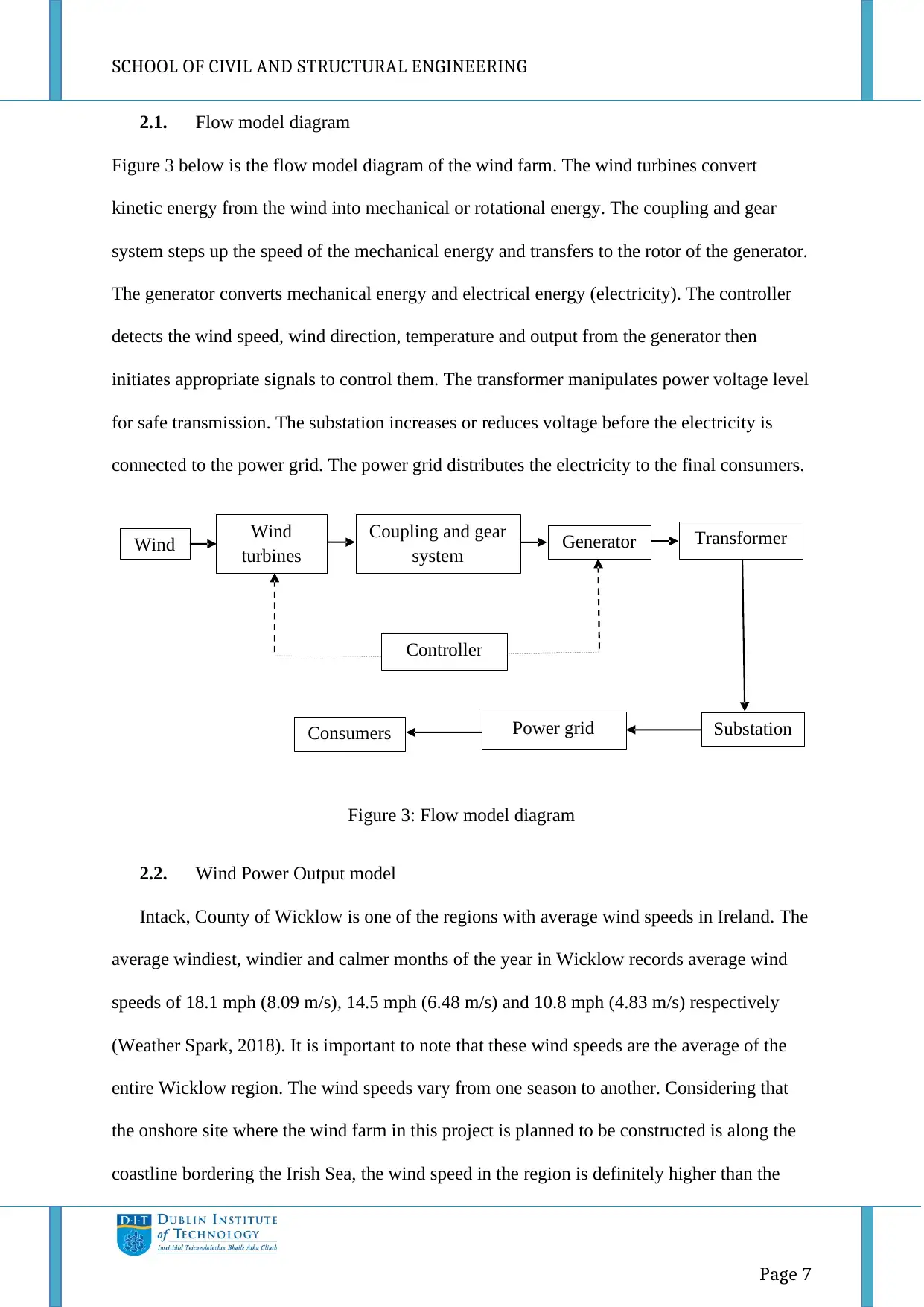
Document Page
SCHOOL OF CIVIL AND STRUCTURAL ENGINEERING
Page 43
1
1
81334
5
3298
00
849
720
0
162
669
0
654071
0
98110
6.5
63729
48.5
0.49
0
31227
11
3224
4107.
23
56
01
35
1
2
81334
5
3298
00
849
720
0
162
669
0
654071
0
98110
6.5
63729
48.5
0.45
9
29266
27
3517
0734.
23
52
49
62.
5
1
3
81334
5
3298
00
849
720
0
162
669
0
654071
0
98110
6.5
63729
48.5
0.43
0
27428
56
3791
3589.
91
49
19
98.
6
1
4
81334
5
3298
00
849
720
0
162
669
0
654071
0
98110
6.5
63729
48.5
0.40
3
25706
24
4048
4213.
79
46
11
04.
6
1
5
81334
5
3298
00
849
720
0
162
669
0
654071
0
98110
6.5
63729
48.5
0.37
8
24092
07
4289
3420.
79
43
21
50.
5
1
6
81334
5
3298
00
849
720
0 0
816740
0
12251
10
61289
45
0.35
4
21714
76
4506
4896.
69
40
50
14.
5
1
7
81334
5
3298
00
849
720
0 0
816740
0
12251
10
61289
45
0.33
2
20351
23
4710
0019.
37
37
95
82.
5
1
8
81334
5
3298
00
849
720
0 0
816740
0
12251
10
61289
45
0.31
1
19073
31
4900
7350.
84
35
57
47.
4
1
9
81334
5
3298
00
849
720
0 0
816740
0
12251
10
61289
45
0.29
2
17875
65
5079
4915.
48
33
34
09
2
0
81334
5
3298
00
849
720
0 0
816740
0
12251
10
61289
45
0.27
3
16753
18
5247
0233.
79
31
24
73.
3
32533
800
6596
000
169
944
000
244
003
50
138947
650
20842
148
10997
2052.
5 NPV
52470
234
28
66
49
85
Document Page
SCHOOL OF CIVIL AND STRUCTURAL ENGINEERING
Page 44
Appendix 4: Summary of calculations for scenario 3
Y
e
a
r
Invest
ment
costs
(€)
O&
M
Cost
s (€)
Rev
enu
es
(€)
Dep
reci
atio
n
Net
taxable
income
(€)
Corpo
ration
tax (€)
After
tax
cash
flow
Disco
unt
facto
r
Prese
nt
Value
(PV)
Cum
mulat
ive
PV
PV
(co
sts)
0
11640
000 0 0 0 0 0
-
11640
000
1.00
0
-
1.2E+0
7
-
1164
0000
11
64
00
00
1
58200
0
2425
00
127
458
00
582
000
119213
00
17881
95
10133
105
0.91
1
92286
93
-
2411
306.9
22
75
09
10.
7
2
58200
0
2425
00
127
458
00
582
000
119213
00
17881
95
10133
105
0.82
9
84050
03
5993
695.8
82
68
38
89.
6
3
58200
0
2425
00
127
458
00
582
000
119213
00
17881
95
10133
105
0.75
5
76548
30
1364
8525.
39
62
28
50.
2
4
58200
0
2425
00
127
458
00
582
000
119213
00
17881
95
10133
105
0.68
8
69716
12
2062
0136.
97
56
72
58.
9
5
58200
0
2425
00
127
458
00
582
000
119213
00
17881
95
10133
105
0.62
7
63493
73
2696
9509.
99
51
66
29.
2
6
58200
0
2425
00
127
458
00
582
000
119213
00
17881
95
10133
105
0.57
1
57826
71
3275
2181.
23
47
05
18.
4
7
58200
0
2425
00
127
458
00
582
000
119213
00
17881
95
10133
105
0.52
0
52665
49
3801
8730.
63
42
85
23.
1
8
58200
0
2425
00
127
458
00
582
000
119213
00
17881
95
10133
105
0.47
3
47964
93
4281
5223.
71
39
02
76.
1
9
58200
0
2425
00
127
458
00
582
000
119213
00
17881
95
10133
105
0.43
1
43683
91
4718
3614.
49
35
54
42.
7
1 58200 2425 127 582 119213 17881 10133 0.39 39784 5116 32
Document Page
SCHOOL OF CIVIL AND STRUCTURAL ENGINEERING
Page 45
0 0 00 458
00
000 00 95 105 3 98 2112.
46
37
18.
3
1
1
58200
0
2425
00
127
458
00
582
000
119213
00
17881
95
10133
105
0.35
8
36234
04
5478
5516.
82
29
48
25.
4
1
2
58200
0
2425
00
127
458
00
582
000
119213
00
17881
95
10133
105
0.32
6
33000
04
5808
5520.
78
26
85
11.
3
1
3
58200
0
2425
00
127
458
00
582
000
119213
00
17881
95
10133
105
0.29
7
30054
68
6109
0988.
87
24
45
45.
8
1
4
58200
0
2425
00
127
458
00
582
000
119213
00
17881
95
10133
105
0.27
0
27372
20
6382
8209.
35
22
27
19.
3
1
5
58200
0
2425
00
127
458
00
582
000
119213
00
17881
95
10133
105
0.24
6
24929
15
6632
1124.
18
20
28
40.
9
1
6
58200
0
2425
00
127
458
00 0
125033
00
18754
95
10045
805
0.22
4
22508
54
6857
1978.
06
18
47
36.
7
1
7
58200
0
2425
00
127
458
00 0
125033
00
18754
95
10045
805
0.20
4
20499
58
7062
1936.
05
16
82
48.
4
1
8
58200
0
2425
00
127
458
00 0
125033
00
18754
95
10045
805
0.18
6
18669
93
7248
8928.
76
15
32
31.
7
1
9
58200
0
2425
00
127
458
00 0
125033
00
18754
95
10045
805
0.16
9
17003
58
7418
9286.
42
13
95
55.
3
2
0
58200
0
2425
00
127
458
00 0
125033
00
18754
95
10045
805
0.15
4
15485
95
7573
7881.
74
12
70
99.
5
23280
000
4850
000
254
916
000
873
000
0
241336
000
36200
400
19058
5600 NPV
75737
882
18
75
63

Secure Best Marks with AI Grader

Need help grading? Try our AI Grader for instant feedback on your assignments.
Document Page
SCHOOL OF CIVIL AND STRUCTURAL ENGINEERING
Page 46
32
Appendix 5: Summary of calculations for scenario 4
Y
e
a
r
Invest
ment
costs
(€)
O&
M
Cost
s (€)
Rev
enu
es
(€)
Dep
reci
atio
n
Net
taxable
income
(€)
Corpo
ration
tax (€)
After
tax
cash
flow
Disco
unt
facto
r
Prese
nt
Value
(PV)
Cum
mulat
ive
PV
PV
(co
sts)
0
16266
900 0 0 0 0 0
-
16266
900
1.00
0
-
16266
900
-
1626
6900
16
26
69
00
1
81334
5
3298
00
127
458
00
162
669
0
107893
10
16183
97
99842
58.5
0.87
5
87351
34.29
6
-
7531
765.7
04
10
00
12
7
2
81334
5
3298
00
127
458
00
162
669
0
107893
10
16183
97
99842
58.5
0.76
5
76422
87.22
3
1105
21.51
86
87
50
01.
6
3
81334
5
3298
00
127
458
00
162
669
0
107893
10
16183
97
99842
58.5
0.67
0
66861
65.54
9
6796
687.0
68
76
55
30.
7
4
81334
5
3298
00
127
458
00
162
669
0
107893
10
16183
97
99842
58.5
0.58
6
58496
63.64
8
1264
6350.
72
66
97
55.
7
5
81334
5
3298
00
127
458
00
162
669
0
107893
10
16183
97
99842
58.5
0.51
3
51178
15.96
5
1776
4166.
68
58
59
63
6
81334
5
3298
00
127
458
00
162
669
0
107893
10
16183
97
99842
58.5
0.44
8
44775
29.27
8
2224
1695.
96
51
26
53.
5
7
81334
5
3298
00
127
458
00
162
669
0
107893
10
16183
97
99842
58.5
0.39
2
39173
48.45
2615
9044.
41
44
85
15.
8
8
81334
5
3298
00
127
458
00
162
669
0
107893
10
16183
97
99842
58.5
0.34
3
34272
51.48
7
2958
6295.
89
39
24
02.
2
9
81334
5
3298
00
127
458
162
669
107893
10
16183
97
99842
58.5
0.30
0
29984
70.24
3258
4766.
34
33
Document Page
SCHOOL OF CIVIL AND STRUCTURAL ENGINEERING
Page 47
00 0 2 14 09
1
0
81334
5
3298
00
127
458
00
162
669
0
107893
10
16183
97
99842
58.5
0.26
3
26233
33.54
5
3520
8099.
68
30
03
57.
9
1
1
81334
5
3298
00
127
458
00
162
669
0
107893
10
16183
97
99842
58.5
0.23
0
22951
29.96
1
3750
3229.
64
26
27
80.
3
1
2
81334
5
3298
00
127
458
00
162
669
0
107893
10
16183
97
99842
58.5
0.20
1
20079
87.71
7
3951
1217.
36
22
99
04
1
3
81334
5
3298
00
127
458
00
162
669
0
107893
10
16183
97
99842
58.5
0.17
6
17567
69.65
6
4126
7987.
02
20
11
40.
9
1
4
81334
5
3298
00
127
458
00
162
669
0
107893
10
16183
97
99842
58.5
0.15
4
15369
81.32
7
4280
4968.
34
17
59
76.
3
1
5
81334
5
3298
00
127
458
00
162
669
0
107893
10
16183
97
99842
58.5
0.13
5
13446
90.57
5
4414
9658.
92
15
39
60
1
6
81334
5
3298
00
127
458
00 0
124160
00
18624
00
97402
55
0.11
8
11477
05.97
4529
7364.
89
13
46
98.
2
1
7
81334
5
3298
00
127
458
00 0
124160
00
18624
00
97402
55
0.10
3
10041
17.20
9
4630
1482.
1
11
78
46.
2
1
8
81334
5
3298
00
127
458
00 0
124160
00
18624
00
97402
55
0.09
0
87849
2.746
4717
9974.
84
10
31
02.
5
1
9
81334
5
3298
00
127
458
00 0
124160
00
18624
00
97402
55
0.07
9
76858
5.079
6
4794
8559.
92
90
20
3.4
1
2
0
81334
5
3298
00
127
458
00 0
124160
00
18624
00
97402
55
0.06
9
67242
7.891
2
4862
0987.
81
78
91
8.1
2
32533
800
6596
000
254
916
000
244
003
50
223919
650
33587
948
18219
8252.
5 NPV
48620
987.8
1
23
70
90
Document Page
SCHOOL OF CIVIL AND STRUCTURAL ENGINEERING
Page 48
46
Appendix 6: Summary of calculations for scenario 5
Y
e
a
r
Invest
ment
costs
(€)
O&
M
Cost
s (€)
Rev
enu
es
(€)
Dep
reci
atio
n
Net
taxable
income
(€)
Corpo
ration
tax (€)
After
tax
cash
flow
Disco
unt
facto
r
Prese
nt
Value
(PV)
Cum
mulat
ive
PV
PV
(co
sts)
0
49806
900 0 0 0 0 0
-
49806
900
1.00
0
-
49806
900
-
4980
6900
49
80
69
00
1
24903
45
7425
00
520
344
00
498
069
0
463112
10
69466
82
41854
873.5
0.91
1
38119
192.6
2
-
1168
7707.
38
29
44
30
3
2
24903
45
7425
00
520
344
00
498
069
0
463112
10
69466
82
41854
873.5
0.82
9
34716
933.1
7
2302
9225.
8
26
81
51
5
3
24903
45
7425
00
520
344
00
498
069
0
463112
10
69466
82
41854
873.5
0.75
5
31618
336.2
2
5464
7562.
02
24
42
18
1
4
24903
45
7425
00
520
344
00
498
069
0
463112
10
69466
82
41854
873.5
0.68
8
28796
298.9
3
8344
3860.
94
22
24
20
9
5
24903
45
7425
00
520
344
00
498
069
0
463112
10
69466
82
41854
873.5
0.62
7
26226
137.4
6
1096
6999
8.4
20
25
69
1
6
24903
45
7425
00
520
344
00
498
069
0
463112
10
69466
82
41854
873.5
0.57
1
23885
371.0
9
1335
5536
9.5
18
44
89
2
7
24903
45
7425
00
520
344
00
498
069
0
463112
10
69466
82
41854
873.5
0.52
0
21753
525.5
8
1553
0889
5.1
16
80
22
9
8
24903
45
7425
00
520
344
00
498
069
0
463112
10
69466
82
41854
873.5
0.47
3
19811
954.0
8
1751
2084
9.2
15
30
26
3

Paraphrase This Document

Need a fresh take? Get an instant paraphrase of this document with our AI Paraphraser
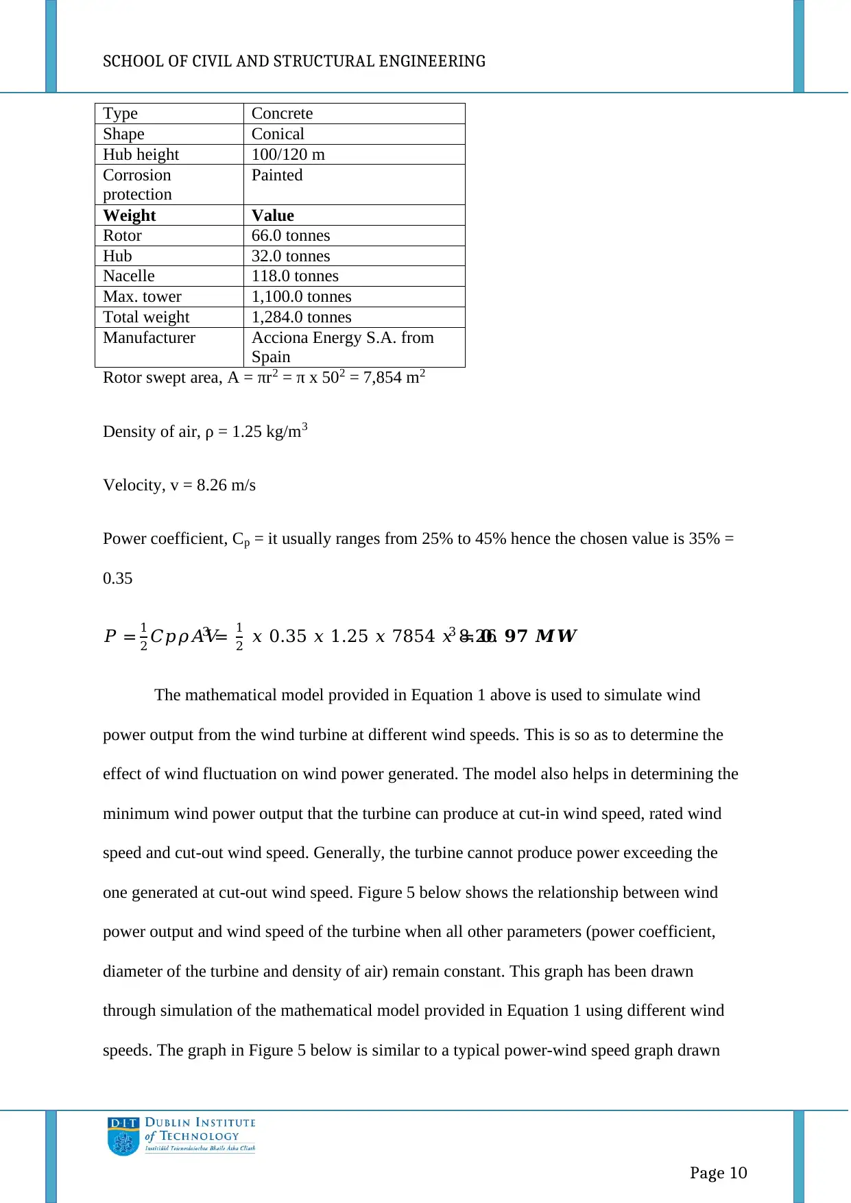
Document Page
SCHOOL OF CIVIL AND STRUCTURAL ENGINEERING
Page 49
9
24903
45
7425
00
520
344
00
498
069
0
463112
10
69466
82
41854
873.5
0.43
1
18043
674.0
3
1931
6452
3.2
13
93
68
2
1
0
24903
45
7425
00
520
344
00
498
069
0
463112
10
69466
82
41854
873.5
0.39
3
16433
218.6
2095
9774
1.8
12
69
29
2
1
1
24903
45
7425
00
520
344
00
498
069
0
463112
10
69466
82
41854
873.5
0.35
8
14966
501.4
6
2245
6424
3.3
11
56
00
3
1
2
24903
45
7425
00
520
344
00
498
069
0
463112
10
69466
82
41854
873.5
0.32
6
13630
693.5
2381
9493
6.7
10
52
82
6
1
3
24903
45
7425
00
520
344
00
498
069
0
463112
10
69466
82
41854
873.5
0.29
7
12414
110.6
5
2506
0904
7.4
95
88
58.
4
1
4
24903
45
7425
00
520
344
00
498
069
0
463112
10
69466
82
41854
873.5
0.27
0
11306
111.7
1
2619
1515
9.1
87
32
77.
2
1
5
24903
45
7425
00
520
344
00
498
069
0
463112
10
69466
82
41854
873.5
0.24
6
10297
005.2
2722
1216
4.3
79
53
34.
4
1
6
24903
45
7425
00
520
344
00 0
512919
00
76937
85
41107
770
0.22
4
92105
69.33
4
2814
2273
3.6
72
43
48.
3
1
7
24903
45
7425
00
520
344
00 0
512919
00
76937
85
41107
770
0.20
4
83884
96.66
2
2898
1123
0.3
65
96
97.
9
1
8
24903
45
7425
00
520
344
00 0
512919
00
76937
85
41107
770
0.18
6
76397
96.59
5
2974
5102
6.9
60
08
17.
8
1
9
24903
45
7425
00
520
344
00 0
512919
00
76937
85
41107
770
0.16
9
69579
20.39
6
3044
0894
7.3
54
71
92.
9
2
0
24903
45
7425
00
520
344 0
512919
00
76937
85
41107
770
0.15
4
63369
03.82
3107
4585
49
83
Document Page
SCHOOL OF CIVIL AND STRUCTURAL ENGINEERING
Page 50
00 2 1.1 54.
2
99613
800
1485
0000
104
068
800
0
747
103
50
951127
650
1.43E+
08
78355
5052.
5 NPV
31074
5851.
1
77
70
98
68
Document Page
SCHOOL OF CIVIL AND STRUCTURAL ENGINEERING
Page 51

Secure Best Marks with AI Grader

Need help grading? Try our AI Grader for instant feedback on your assignments.
Document Page
SCHOOL OF CIVIL AND STRUCTURAL ENGINEERING
Page 52
Document Page
SCHOOL OF CIVIL AND STRUCTURAL ENGINEERING
Page 53
1 out of 54
circle_padding
hide_on_mobile
zoom_out_icon
[object Object]

Your All-in-One AI-Powered Toolkit for Academic Success.

Available 24*7 on WhatsApp / Email

[object Object]