Windows User Windows User Risk Management List of Figures 2 Question 1 3 1.1 Introduction 3 1.2 Decision Tree 5 1.3 Decision Tree with EVM 6 1.4 Discussion and calculation 7 61.5 Bayes Rule Outcomes 9

Windows User | Windows User Risk management List of figures 2 Question 1 3 1.1 Introduction 3 1.2 Decision Tree 5 1.3 Decision Tree with EVM 6 1.4 Discussion and calculation 7 61.5 Bayes Rule Problem 9 1.6 Bayes Rule Outcomes 10 2.0 Question 2 11 2.1 Objective 11 2.2 Original Data 11 2.3 First Alteration with Discussion 12 2.4 Second Alteration and Discussion 13 2.5 Final Alteration and Discussion 14 3.0 Question 3 16 3.1 Problem statement 16 3.2 Constraints 16 3.3 Objectives 16 3.4 Equations 16 3.5 Coordinates

1 | P a g e
Windows User

Risk management
Table of Contents
List of figures................................................................................................................2
Question 1....................................................................................................................3
1.1 Introduction......................................................................................................3
1.2 Decision Tree......................................................................................................5
1.3 Decision Tree with EVM......................................................................................6
1.4 Discussion and calculation..................................................................................7
61.5 Bayes Rule Problem..........................................................................................9
1.6 Bayes Rule Outcomes......................................................................................10
2.0 Question 2............................................................................................................11
2.1 Objective............................................................................................................11
2.2 Original Data.....................................................................................................11
2.3 First Alteration with Discussion.........................................................................12
2.4 Second Alteration and Discussion....................................................................13
2.5 Final Alteration and Discussion.........................................................................14
3.0 Question 3............................................................................................................16
3.1 Problem statement............................................................................................16
3.2 Constraints........................................................................................................16
3.3 Objectives..........................................................................................................16
3.4 Equations..........................................................................................................16

3.5 Coordinates.......................................................................................................18
3.6 Graphical Illustration..........................................................................................19
3.6 Final number.....................................................................................................19
3.7 Spreadsheet solution........................................................................................20
4.0 Question 4...........................................................................................................21
4.1 Expected Activity...............................................................................................21
4.2 Excel model.......................................................................................................22
4.3 Network Diagram...............................................................................................23
4.4 Z value/ project finishing before 46 weeks........................................................23
4.5 Project lasting longer than 46 weeks................................................................24
4.6 Completion of project time where 85% of the project is complete....................24
4.7 Project Risk Exposure.......................................................................................24
Question 5..................................................................................................................26
Network project.......................................................................................................26
Appendices.................................................................................................................27

List of figures
Figure 1: Decision tree produced in Visio.....................................................................2
Figure 2: Decision Tree with EVM................................................................................3
Figure 3: Original excel model......................................................................................8
Figure 4: shows the excel model 2 with alteration.......................................................9
Figure 5: Shows excel 3 model with alteration...........................................................10
Figure 6: Shows the final excel model with alterations..............................................11
Figure 7 shows the illustration of Constraints.............................................................16
Figure 8 shows the spreadsheet solution with solver.................................................17
Figure 9 shows the Excel Model and PERT analysis.................................................19
Figure 10 Network diagram with critical path.............................................................20
Figure 11 shows the critical path for the project.........................................................20
Figure 12 Network Project..........................................................................................23

Question 1
1.1 Introduction
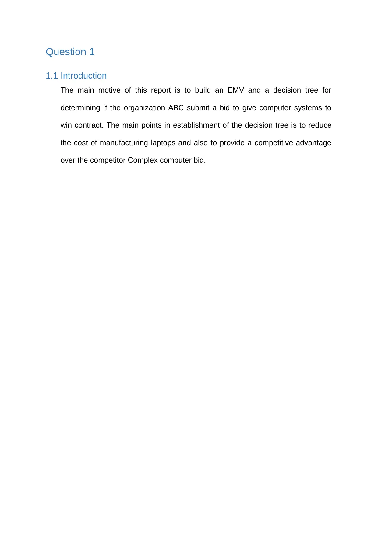
The main motive of this report is to build an EMV and a decision tree for
determining if the organization ABC submit a bid to give computer systems to
win contract. The main points in establishment of the decision tree is to reduce
the cost of manufacturing laptops and also to provide a competitive advantage
over the competitor Complex computer bid.

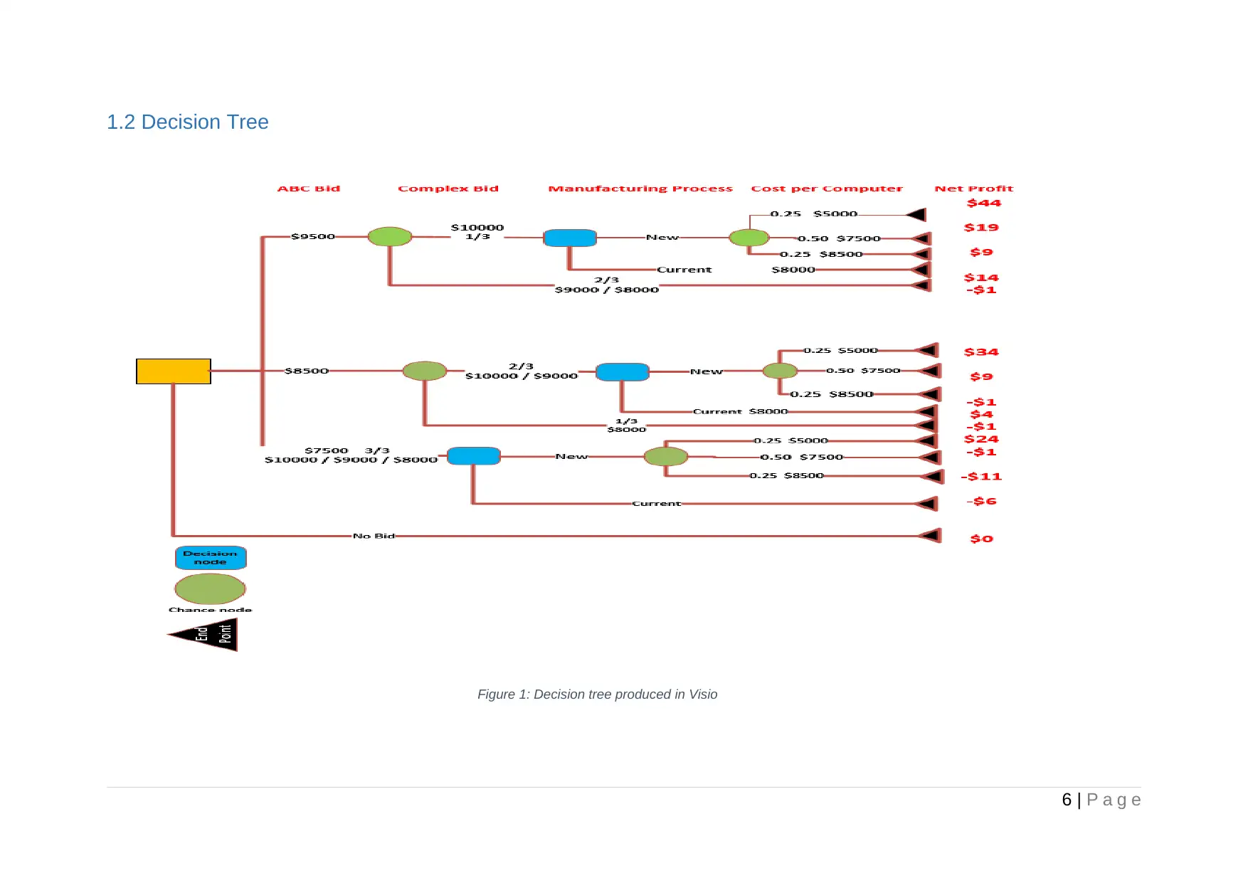
1.2 Decision Tree
6 | P a g e
Figure 1: Decision tree produced in Visio

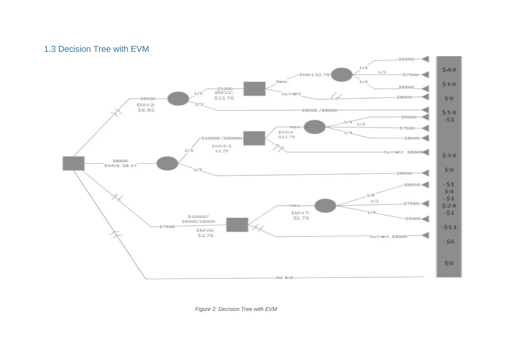
1.3 Decision Tree with EVM
Figure 2: Decision Tree with EVM

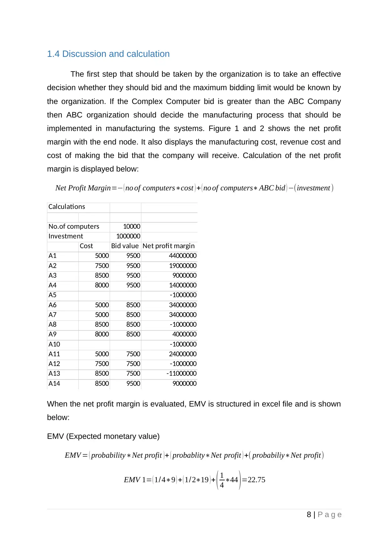
1.4 Discussion and calculation
The first step that should be taken by the organization is to take an effective
decision whether they should bid and the maximum bidding limit would be known by
the organization. If the Complex Computer bid is greater than the ABC Company
then ABC organization should decide the manufacturing process that should be
implemented in manufacturing the systems. Figure 1 and 2 shows the net profit
margin with the end node. It also displays the manufacturing cost, revenue cost and
cost of making the bid that the company will receive. Calculation of the net profit
margin is displayed below:
Net Profit Margin=− ( no of computers∗cost ) + ( no of computers∗ABC bid ) −(investment )
Calculations
No.of computers 10000
Investment 1000000
Cost Bid value Net profit margin
A1 5000 9500 44000000
A2 7500 9500 19000000
A3 8500 9500 9000000
A4 8000 9500 14000000
A5 -1000000
A6 5000 8500 34000000
A7 5000 8500 34000000
A8 8500 8500 -1000000
A9 8000 8500 4000000
A10 -1000000
A11 5000 7500 24000000
A12 7500 7500 -1000000
A13 8500 7500 -11000000
A14 8500 9500 9000000
When the net profit margin is evaluated, EMV is structured in excel file and is shown
below:
EMV (Expected monetary value)
EMV = ( probability∗Net profit ) + ( probablity∗Net profit ) +( probabiliy∗Net profit)
EMV 1= ( 1/4∗9 ) + ( 1/2∗19 )+ ( 1
4 ∗44 )=22.75
8 | P a g e

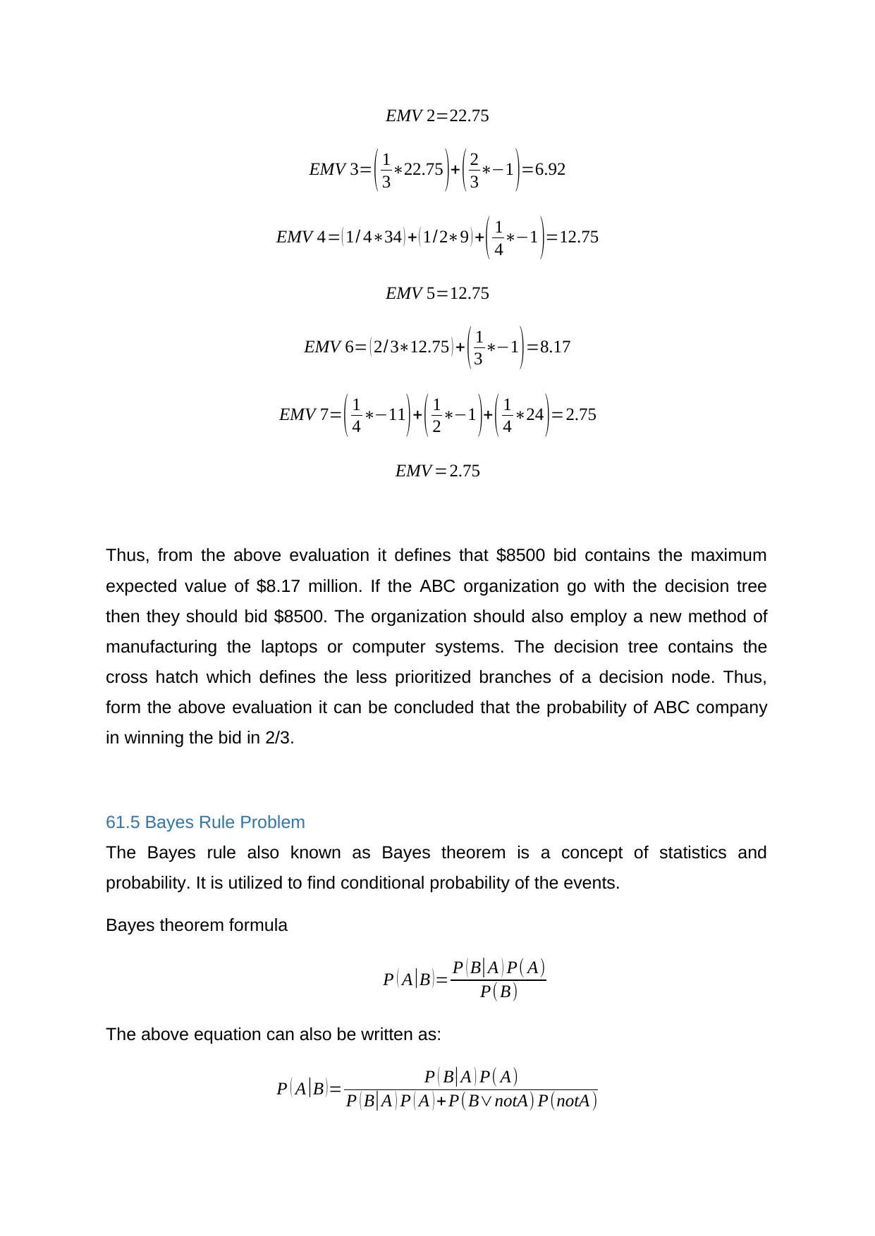
EMV 2=22.75
EMV 3= ( 1
3∗22.75 )+ ( 2
3∗−1 )=6.92
EMV 4= ( 1/ 4∗34 ) + ( 1/2∗9 ) +( 1
4∗−1 )=12.75
EMV 5=12.75
EMV 6= ( 2/3∗12.75 ) + ( 1
3 ∗−1)=8.17
EMV 7= ( 1
4 ∗−11 )+ ( 1
2∗−1 )+ ( 1
4 ∗24 )=2.75
EMV =2.75
Thus, from the above evaluation it defines that $8500 bid contains the maximum
expected value of $8.17 million. If the ABC organization go with the decision tree
then they should bid $8500. The organization should also employ a new method of
manufacturing the laptops or computer systems. The decision tree contains the
cross hatch which defines the less prioritized branches of a decision node. Thus,
form the above evaluation it can be concluded that the probability of ABC company
in winning the bid in 2/3.
61.5 Bayes Rule Problem
The Bayes rule also known as Bayes theorem is a concept of statistics and
probability. It is utilized to find conditional probability of the events.
Bayes theorem formula
P ( A |B )= P ( B|A ) P( A)
P( B)
The above equation can also be written as:
P ( A |B )= P ( B|A ) P( A)
P ( B|A ) P ( A ) +P(B∨notA) P(notA )

Where
P (A) is the probability of the event A
P (B) is the probability of the event B
P (A | B) is the probability of the event A happening given that the event B has
already happened
P (B | A) is the probability of the event B happening given that the event A has
already happened
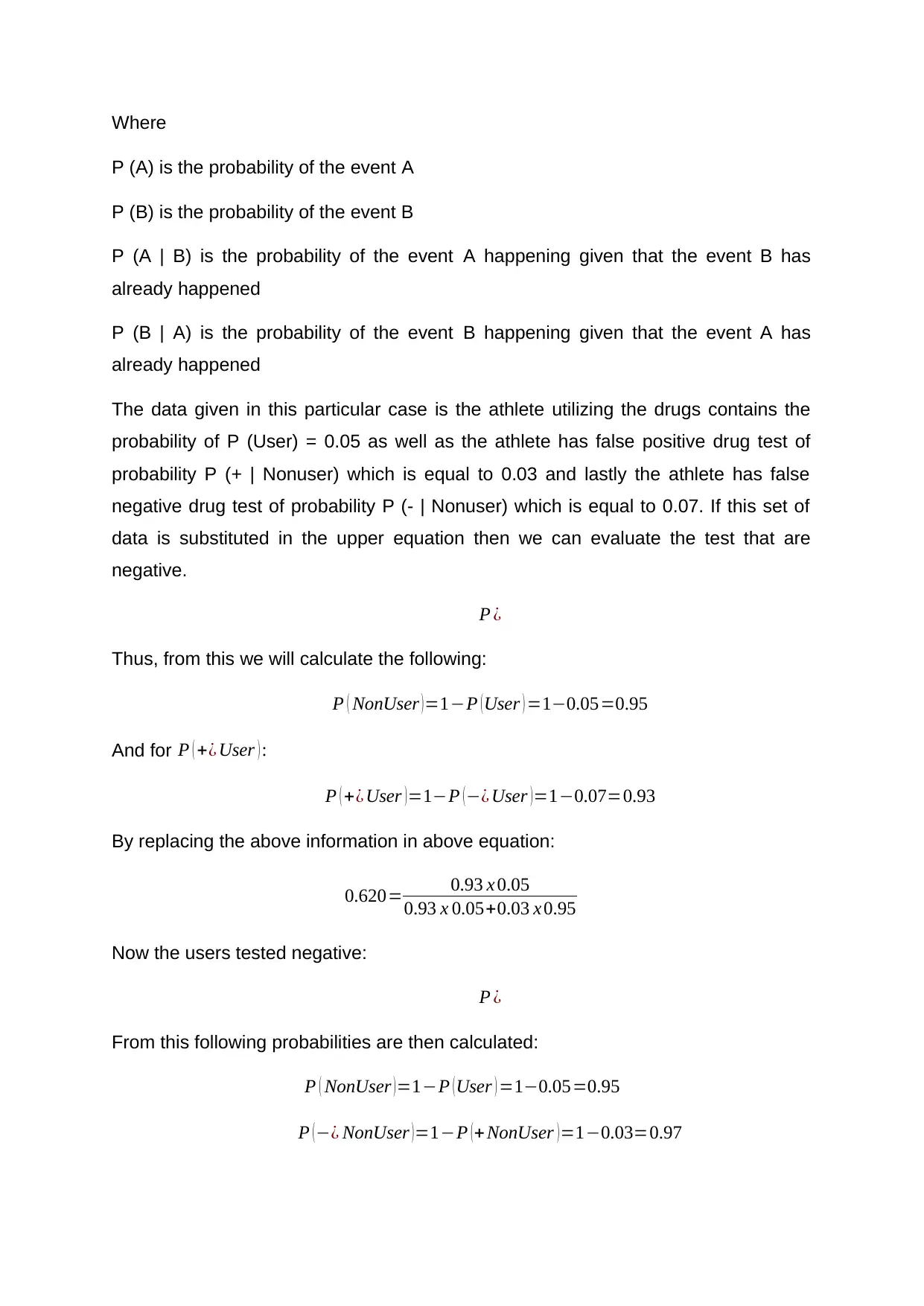
The data given in this particular case is the athlete utilizing the drugs contains the
probability of P (User) = 0.05 as well as the athlete has false positive drug test of
probability P (+ | Nonuser) which is equal to 0.03 and lastly the athlete has false
negative drug test of probability P (- | Nonuser) which is equal to 0.07. If this set of
data is substituted in the upper equation then we can evaluate the test that are
negative.
P ¿
Thus, from this we will calculate the following:
P ( NonUser )=1−P (User ) =1−0.05=0.95
And for P ( +¿ User ) :
P ( +¿ User )=1−P (−¿ User )=1−0.07=0.93
By replacing the above information in above equation:
0.620= 0.93 x 0.05
0.93 x 0.05+0.03 x 0.95
Now the users tested negative:
P ¿
From this following probabilities are then calculated:
P ( NonUser )=1−P (User ) =1−0.05=0.95
P (−¿ NonUser )=1−P (+ NonUser )=1−0.03=0.97

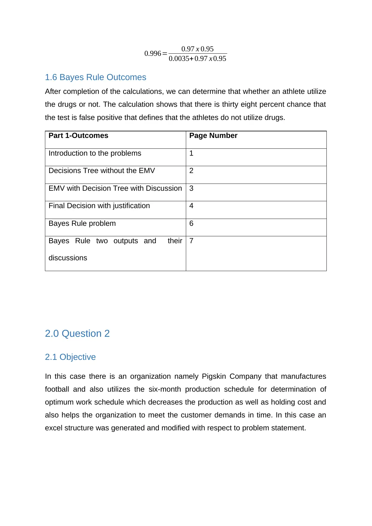
0.996= 0.97 x 0.95
0.0035+ 0.97 x 0.95
1.6 Bayes Rule Outcomes
After completion of the calculations, we can determine that whether an athlete utilize
the drugs or not. The calculation shows that there is thirty eight percent chance that
the test is false positive that defines that the athletes do not utilize drugs.
Part 1-Outcomes Page Number
Introduction to the problems 1
Decisions Tree without the EMV 2
EMV with Decision Tree with Discussion 3
Final Decision with justification 4
Bayes Rule problem 6
Bayes Rule two outputs and their
discussions
7
2.0 Question 2
2.1 Objective
In this case there is an organization namely Pigskin Company that manufactures
football and also utilizes the six-month production schedule for determination of
optimum work schedule which decreases the production as well as holding cost and
also helps the organization to meet the customer demands in time. In this case an
excel structure was generated and modified with respect to problem statement.

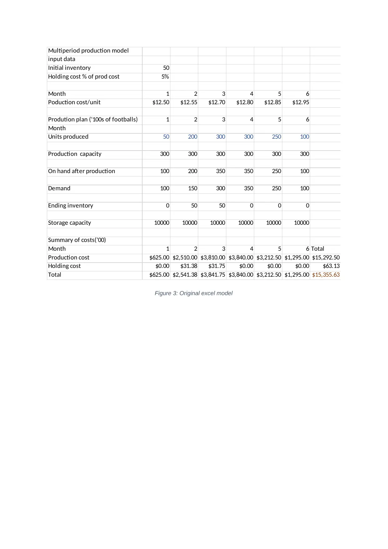
Multiperiod production model
input data
Initial inventory 50
Holding cost % of prod cost 5%
Month 1 2 3 4 5 6
Poduction cost/unit $12.50 $12.55 $12.70 $12.80 $12.85 $12.95
Prodution plan ('100s of footballs) 1 2 3 4 5 6
Month
Units produced 50 200 300 300 250 100
Production capacity 300 300 300 300 300 300
On hand after production 100 200 350 350 250 100
Demand 100 150 300 350 250 100
Ending inventory 0 50 50 0 0 0
Storage capacity 10000 10000 10000 10000 10000 10000
Summary of costs('00)
Month 1 2 3 4 5 6 Total
Production cost $625.00 $2,510.00 $3,810.00 $3,840.00 $3,212.50 $1,295.00 $15,292.50
Holding cost $0.00 $31.38 $31.75 $0.00 $0.00 $0.00 $63.13
Total $625.00 $2,541.38 $3,841.75 $3,840.00 $3,212.50 $1,295.00 $15,355.63
Figure 3: Original excel model

2.2 Original Data
Input variables Initial inventory, production as well as
storage capacities, unit production costs
and percentage of unit holding cost.
Decision variables Monthly production quantities
Other calculated variables Units on hand after production, monthly
production and inventory holding costs and
ending inventories.
Objective cell Total cost
Constraints Ending inventory ≤ storage capacity (each
month)
Units produced ≤ Produced capacity (each
month)

2.3 First Alteration with Discussion
input data
Initial inventory 50
Holding cost % of prod cost 5%
Month 1 2 3 4 5 6
Poduction cost/unit $12.50 $12.55 $12.70 $12.80 $12.85 $12.95
Prodution plan ('100s of footballs) 1 2 3 4 5 6
Month
Units produced 0 0 300 300 300 300
Production capacity 300 300 300 300 300 300
On hand after production 50 50 350 650 950 1250
Demand 1250 1250
Ending inventory 50 50 350 650 950 0
Storage capacity 10000 10000 10000 10000 10000 10000
Summary of costs('00)
Month 1 2 3 4 5 6 Total
Production cost $0.00 $0.00 $3,810.00 $3,840.00 $3,855.00 $3,885.00 $15,390.00
Holding cost $31.25 $31.38 $222.25 $416.00 $610.38 $0.00 $1,311.25
Total $31.25 $31.38 $4,032.25 $4,256.00 $4,465.38 $3,885.00 $16,701.25
Figure 4: shows the excel model 2 with alteration
Figure 4 is the modified model of the original model. The modified parameters are as
follows: expect for 6th month, in order to meet the demand by 6th month and demands
cannot be met by 6th month. In figure 3 we saw the maximum production capacity is
observed in the 3rd and 4th months but in figure 4 we observed that the maximum
production capacity is observed in the 3rd to 6th month. The ending units is increased
up to 950 till the 5th month as the demand of the units was 0 from 1rd month to 5th
month. From the production schedule of the 2nd figure we can say that the production
is 0 from1st month to 2nd month and thus the production cost was also 0 which
reduces the total production cost to $15,390. We observed that holding cost is more

in case of the modified model than the original model it is due to the fact that the
demand was not met from 1st month to 5th month. The total optimization rises the
overall optimal cost by $1346.
2.4 Second Alteration and Discussion
Figure 5 displays modified production model which is designed to meet the demands
in any of first 5 months and the demand of the 6th month should also be met in the
defined time frame. It can be seen in the figure that production cost increases
compared to the 3rd figure as demand was not fulfilled in 1st month and also the
number of the units produced is zero. Thus, the overall holding cost was raised by
$128 which increased the overall optimal cost from $15,355 to $15,573.
input data
Initial inventory 50
Holding cost % of prod cost 5%
Month 1 2 3 4 5 6
Poduction cost/unit $12.50 $12.55 $12.70 $12.80 $12.85 $12.95
Prodution plan ('100s of footballs) 1 2 3 4 5 6
Month
Units produced 0 50 250 300 300 300
Production capacity 300 300 300 300 300 300
On hand after production 50 100 250 400 400 350
Demand 0 100 150 300 350 350
Ending inventory 50 0 100 100 50 0
Storage capacity 10000 10000 10000 10000 10000 10000
Summary of costs('00)
Month 1 2 3 4 5 6 Total
Production cost $0.00 $627.50 $3,175.00 $3,840.00 $3,855.00 $3,885.00 $15,382.50
Holding cost $31.25 $0.00 $63.50 $64.00 $32.13 $0.00 $190.88
Total $31.25 $627.50 $3,238.50 $3,904.00 $3,887.13 $3,885.00 $15,573.38
Figure 5: Shows excel 3 model with alteration

2.5 Final Alteration and Discussion
Figure 6 is modified such that the 70% of productivity is used to fulfil the demand for
a specific month and the rest 30% is used to fulfil the demands of the later months.
In figure 6 units are manufactured every month yet the capacity of productivity is
maximum for 3rd and 4th month to fulfil the demand and allow float time to the orders
to meet the demands. The overall holding cost was obtained at $ 312.35 as 30% of
the production is kept reserved to fulfil the demands of next months. The total
optimal cost is $15,566 in case of 4th figure which is was $ 15,573.38 which is
relatively higher than in figure 5.
input data
Initial inventory 50
Holding cost % of prod cost 5%
Month 1 2 3 4 5 6
Poduction cost/unit $12.50 $12.55 $12.70 $12.80 $12.85 $12.95
Prodution plan ('100s of footballs) 1 2 3 4 5 6
Month
Units produced 72 268 300 300 260 0
Units supplied 50 188 210 210 182 0
Carried forward 22 80 90 90 78 0
Production capacity 300 300 300 300 300 300
On hand after production 100 210 350 350 272 100
Demand 100 150 300 350 250 100
Ending inventory 22 140 140 90 100 0
Storage capacity 10000 10000 10000 10000 10000 10000
Summary of costs('00)
Month 1 2 3 4 5 6 Total
Production cost $900.00 $3,363.40 $3,810.00 $3,840.00 $3,341.00 $0.00 $15,254.40
Holding cost $13.75 $87.85 $88.90 $57.60 $64.25 $0.00 $312.35
Total $913.75 $3,451.25 $3,898.90 $3,897.60 $3,405.25 $0.00 $15,566.75
Figure 6: Shows the final excel model with alterations

Part 2-Outcomes Page Number
Provide discussion on company objective? 8
Alternation to the spreadsheets with
demand that need not to be fulfilled on
time, alteration in optimal production
schedule as well as optimal total cost with
discussion
9
Changes to the spreadsheet with demand
to be met in any of first 5 months,
alteration in optimal production schedule
as well as optimal total cost with
discussion
10
70% of the production is used to meet the
demand for a particular month and the rest
30% is used to fulfil the demand of later
months, alteration in optimal production
schedule as well as the optimal total cost
with discussion
11

3.0 Question 3
3.1 Problem statement
Gulf Gulf is the United Arab Emirates based company. It is known for fabricating the
golfing appliances and the demand is huge in this company. It begins the market of
fabricating by having two types of golf sacks, one progressive and a medium sized
upmarket. The main requirement is to determine the number of packs that is to be
fabricated which will provide maximum profit to the organization.
3.2 Constraints
The production manager of the Gulf Gulf provides the constraints that resists number
of the products which can be manufactured for a single bag. The available hours act
as the constraints set for every departments of the company. The available hours are
as follows: 135 hours to pack and inspect, 708 hours to finish the task, 630 hours to
cut and 600 hours to sew the product.
3.3 Objectives
We analyse the case study and can promote the project objective as follows:
 To determine the overall number of the deluxe and standard golf bags
 Determine feasible region
 Determine maximum profit contribution considering the constraints
 Solve the total profit contribution by utilizing solver in excel
3.4 Equations
The optimum number of bags that are to be manufactured for a single product can
be demonstrated as
Number of Bags= Hours Available per Stage
Hours needed by Bag
Thus in the above equation data allocated to the bags for every department can be
replaced in the equation

For cutting and Dyeing
Number of Standard Bag= 630
0.7 =900
Number of Deluxe Bag= 630
1 =630
For Sewing:
Number of Standard Bag= 600
0.5 =1200
Number of Deluxe Bag= 600
0.8333 =720
For Finishing:
Number of Standard Bag=708
1 =708
Number of Deluxe Bag= 708
0.6666 =1062
For Inspection and Packaging:
Number of Standard Bag=135
0.1 =1350
Number of Deluxe Bag= 135
0.25 =54

3.5 Coordinates
Constraint
Cutting and Dyeing
S 0 900
D 630 0
Sewing
S 0 1200
D 720 0
Finishing
S 0 708
D 1062 0
Inspection and Packaging
S 0 1350
D 540 0
Total Available Time
S 0 903.04
D 755.27 0
The constraints can be illustrated by creating the graph which can be made by
inputting the data. The X-axis of the graph will depict the Standard Bag and
the Y-axis depicts the deluxe bags. The data is inputted to evaluate the
equation for every line.
Cutting∧Dyeing : y=−1.43 x+900

Sewing : y=−1.67 x +1200
Finishing : y=−0.67 x+708
Inspection∧Packaging : y=−2.5 x +1350
3.6 Graphical Illustration
Figure 7 shows the illustration of Constraints
3.6 Final number
After the successful analysis of the data, it can be said that the Gulf Gulf can gain
the maximum profit by selling 540 standards bags and 252 deluxe bags. By selling
this particular number of units the company can gain a profit of $7668 which is
evaluated by the solver.
3.7 Spreadsheet solution
The spreadsheet which is used to evaluate the above case is shown below:

Golf bag production
Golf bag Standard bag Deluxe Bag Total Sign
Number of bags 540 252 792
Production time
Cutting and dyeing 378 252 630 <= 630
Sewing 270 210 480 <= 600
Finishing 540 168 708 <= 708
Inspection and packaging 54 63 117 <= 135
Revenue
Unit price $10.00 $9.00
Profit $5,400.00 $2,268.00 $7,668.00
Part 3-Outcomes Page Number
Problem statement 13
Discussion data, objectives and
constraints type
13,14
Analytical equations with the condition
forms
14
Graphical representation with Co-
ordinates for the graphs, Feasible
region hatching
16
Final number of standard as well as
deluxe bags with justification
15
Spread sheet model with solver solution 17
4.0 Question 4
4.1 Expected Activity
The predictable operation time is calculated by other variables like total float,
variance and the Standard deviation of the project. The above mentioned factors can
be calculated by the following equations:
Figure 8 shows the spreadsheet solution with solver

Expected Time
¿ Optimistic Duration + ( 6 x Likely Duration ) +Pessimistic Duration
6
Standard Deviation
¿ Pessimistic Duration−Optimistic Duration
6
Variance
¿ Standard Deviation2
Float
¿ Late Finish−Early Finish
4.2 Excel model
Activity code Activity
Optimistic
duration
Most likely
duration
Pessimistic
duration
Immediatepr
edecessor
Expected
time SD Variance
Early
start Late start
Early
finish
Late
finish Float
Critical
path
mean pof
project
SD of
project
A
Set up the project acquisition
team 1 2 3 2 0.3333 0.111089 0 0 2 2 0 Yes 2 0.1111
B
Write down the software
requirements 1 2 3 A 2 0.3333 0.111089 2 2 4 4 0 Yes 2 0.1111
C
develop a contractor evalaution
grid that will be used to evakuate
proposals 0.5 1 1.5 B 1 0.1667 0.027789 4 7 5 8 3 0 0
D
Identify and select potential
contractors 0.5 1 1.5 A 1 0.1667 0.027789 2 3 3 4 1 0 0
E
Develop and send out a request
for proposal to potential
contractors 3 4 5 B,D 4 0.3333 0.111089 4 4 8 8 0 Yes 4 0.1111
F
Audit candidate contractors,
select one contractor, negotiate
and sign an agreement 1 2 3 C,E 2 0.3333 0.111089 8 8 10 10 0 Yes 2 0.1111
G
Prepare the definition of
functional specifications 3 5 7 F 5 0.6667 0.444489 10 10 15 15 0 Yes 5 0.4444
H Develop a software testing plan 1 2 3 G 2 0.3333 0.111089 15 25 17 27 10 0 0
I Software customization phase I 10 12 14 G 12 0.6667 0.444489 15 15 27 27 0 Yes 12 0.0278
J Purchase and install the hardware 1 2 3 G 2 0.3333 0.111089 15 25 17 27 10 0 0
K Test the first release 0.5 1 1.5 H,I,J 1 0.1667 0.027789 27 27 28 28 0 Yes 1 0.4444
L
Develop a training plan for key
users 0.5 1 1.5 K 1 0.1667 0.027789 28 41 29 42 13 0 0.0278
M Software customization phase II 4 6 8 K 6 0.6667 0.444489 28 28 34 34 0 Yes 6 0
N Test the second release 0.5 1 1.5 M 1 0.1667 0.027789 34 34 35 35 0 Yes 1 0.25
O Train Key users 1 2 3 L,N 2 0.3333 0.111089 35 42 37 44 7 0 0.1111
P Software customization phase II 1.5 3 4.5 N 3 0.5 0.25 35 35 38 38 0 Yes 3 0.4444
Q Test the final release 1 2 3 P 2 0.3333 0.111089 38 38 40 40 0 Yes 2 0.1111
R
Software deployment and project
sign-off 2 4 6 Q 4 0.6667 0.444489 40 40 44 44 0 Yes 4 0.1111
44 1.6245
Thus, it can be said that the overall mean duration of project was 44 days and the
standard deviation of project is 1.6245.
4.3 Network Diagram
The values is used to generate the network diagram containing the critical path of
the overall project. The critical path is also displayed below:
Figure 9 shows the Excel Model and PERT analysis

The
project will be completed within 46 weeks as per the network diagram. The
probability to complete the project within 46 weeks is 85% and is calculated using
the Standard normal probabilities process.
4.4 Z value/ project finishing before 46 weeks
The value of Z is calculated by the following formula:
Z= X−μ
SD
Figure 10 Network diagram with critical path
Figure 11 shows the critical path for the project

Z= 46−44
1.6245 =1.23
4.5 Project lasting longer than 46 weeks
Instead of using 46 days, the project can last up to 47 days. In the case of 47 days
the value of Z is:
Z= 47−44
1.6245 =1.847
When the value of Z is evaluated by the standard normal probabilities procedure and
the probability for greater than 46 is determined and it is 96.71%.
4.6 Completion of project time where 85% of the project is complete
The time taken for the completion of the 85% of the project is determined by the
Standard Normal Probability Chart and is evaluated as 1.0400 and thus approximate
time is calculated from the above equation:
Z= X−μ
SD
1.0400= X−44
1.6245
X =46 weeks
Thus it takes 46 weeks to complete 85% of the project.
4.7 Project Risk Exposure
Every activities of the project comprises of risks. Risk is generally defined as the
possible means of the loss. The risk exposure is the analysis of future attack that can
harm any organization or the project. Thus it is the uncertain condition or event that
may harm the project.
Various risk tools or risk analysis techniques can be used to determine the
risk associating with the project. The constraints help to reduce the impacts of the
risk and also allow the members to handle the risk effectively. The emerging risks

can be identified by monitoring progress reviews and project areas. The stakeholder
analysis tool is also used to decrease the project risk exposure. This particular
process is utilized to sum up the risk management wherever any conflicts are found
in the project. The risk exposure can also be handled by TRL approach (Technology
Readiness Levels). Impact assessment is also conducted to determine the
exposures. The above mentioned techniques or tools can be used to draw the
effective handling measures of the risks associated with the project. The identified
risk will be labelled as per their impact and probability of happening. The labelling will
clearly justify the strength of the risk.
Part 4-Outcomes Page Number
Easy Excel model with demonstration 19
Project Duration, Standard deviation of
the project and mean of the project
18
Probability of previous and greater than
46 weeks
21
The project with 85% completion 21
Project risk exposure 21,22

Appendices
Z table for question 4
Figure 12 Network Project