2-Link 3-DOF Robot Positioning Project: MECH 5503, Carleton University

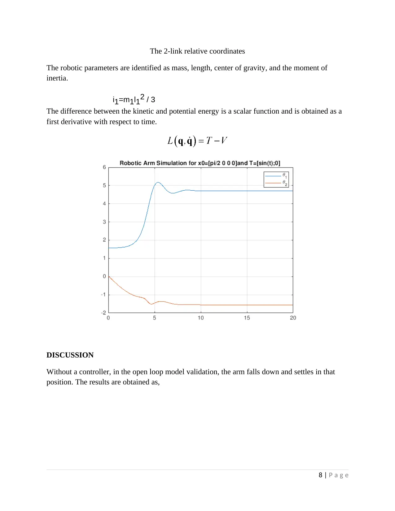
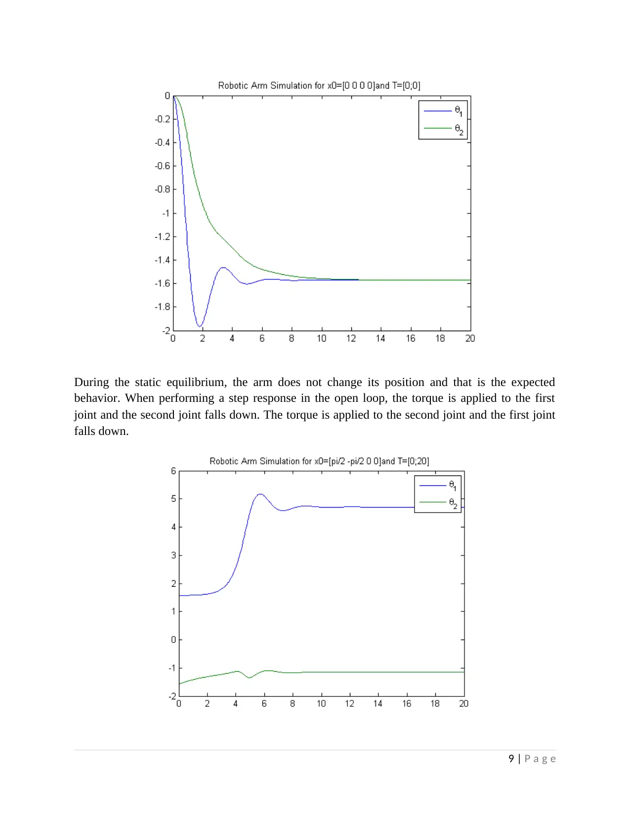
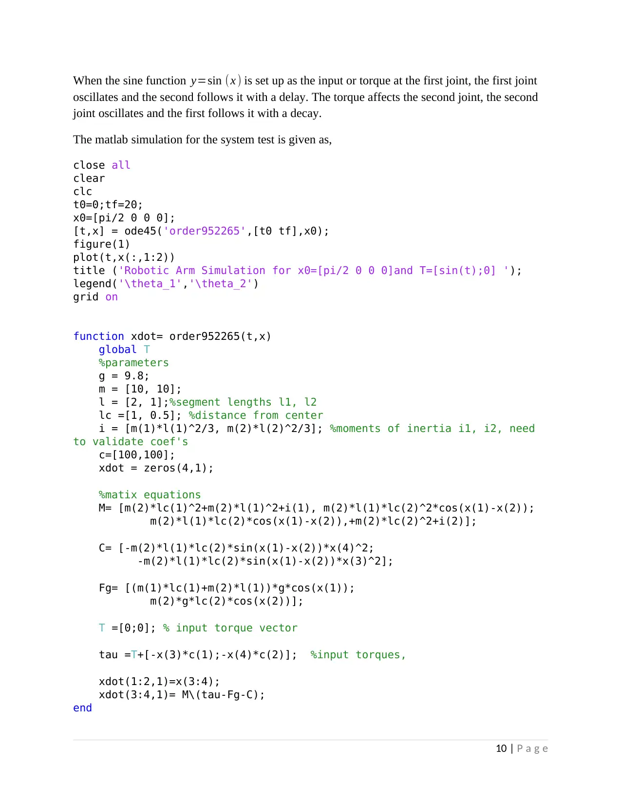
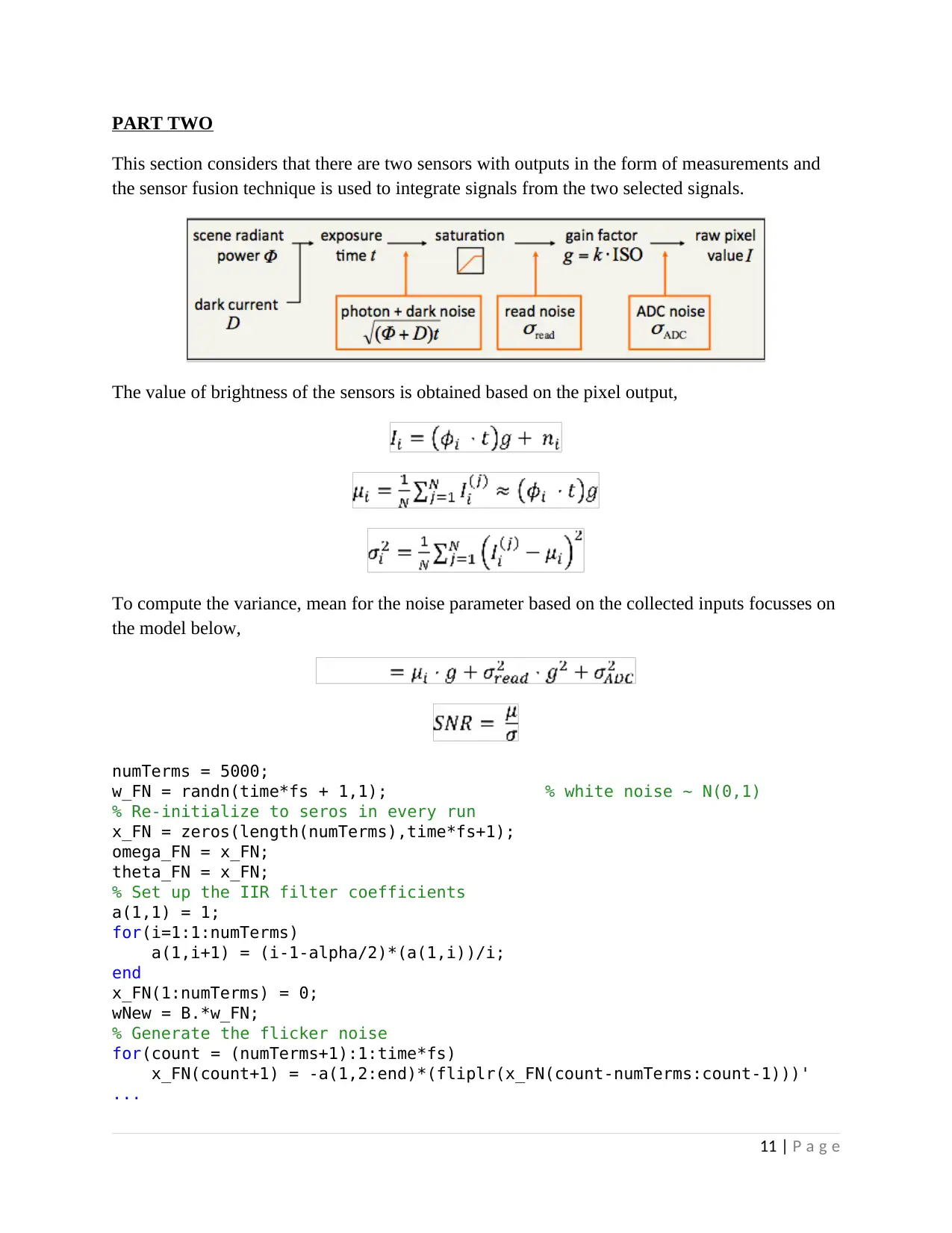
This project focuses on the design and analysis of a control system for a 2-link, 3-DOF robot positioning system, using PI and PD controllers. The project involves deriving torques, linearizing the system, and selecting controller gains. Simulations were performed using Matlab to analyze the robot's response to step and sinusoidal inputs, and for trajectory tracking with a trapezoidal velocity profile. The project also incorporates sensor fusion techniques to integrate signals from two different sensors. The analysis includes forward and inverse kinematics, dynamic equations based on the Lagrangian method, and the identification of key robotic parameters. The results section presents the simulation outcomes, demonstrating the robot's behavior under different control strategies and input conditions. The project concludes with a discussion of the findings and references to relevant literature.

CARLETON UNIVERSITY
DEPARTMENT OF MECHANICAL AND AEROSPACE ENGINEERING
MECH 5503 ROBOTICS
FINAL EXAMINATION PROJECT
STUDENT NAME
STUDENT REGISTRATION NUMBER
DATE OF SUBMISSION
APRIL 11, 2

2-LINK 3-DOF ROBOT POSITIONING BASED ON PI AND PD CONTROLLERS
PART A
INTRODUCTION
Controllers are used to determine or manipulate the action of a mechanical system to ensure it
performs as required. The robotic 2-link arm intends to take some lightweight objects based on
an algorithm stated in the algorithm at the microprocessor. The illustration below shows the 3-
DOF robotic arm,
The robotic arm looks at the high performance, durable, affordable, portable, sustainable, and
easy to operate attributes to ensure that operations run. The robot has a shoulder joint that
enables the rotation of link and the elbow joint rotation. The joints employ specific servomotor to
determine the torque needed for the motion. The section modulus cross-sectional shape of the
robotic arms links and geometries, such as the strength of beams,
S= I
c
The free body diagram of the robotic arm is displayed as the fully stretched out configuration,
1 | P a g e

T elbow= [ Fload∗L2 ] +
[w2∗( L2
2 ) ]
T shoulder= [ Fload∗( L1 +L2 ) + [w2∗( L2
2 + L1 ) ]+ ( wm 3∗L1 ) +( w1∗L1
2 ) ]
The forward kinematics are determined for the five frames of the robotic arm meant to link the
shoulder and the elbow to the load. The defined frames are obtained using the Denavit-
Harternberg (D-H) parameters are determined as,
These D-H parameters are useful in converting the homogenous transform matrices as shown
below,
2 | P a g e

These homogenous transformation matrices are set up in the right order so as to determine the
end-effector frame for the reference frame that is obtained as below,
The Cartesian coordinates of the position of the origin of the end effector frame with respect to
the reference frame,
The procedure of obtaining the analytical expression for the 3 coordinates for the forward
kinematics analysis. The frame assessment free body diagram of the robotic arm is as illustrated
below,
3 | P a g e

The position coordinate equations are used to determine the analytical expressions of the
rotational angles for all the links in the inverse kinematics. The equation is obtained as shown
below,
The results are explicitly expressed as,
The argument is generated for the required quadrant and the robotic arm geometry and
coordinates of the target point are obtained as,
There are a number of assumptions made:
(i) The actuators dynamic is not taken into account.
(ii) The effect of friction forces is assumed to be negligible
(iii) The mass of each link is assumed to be concentrated at the end of each link.
The kinetic energy of the robotic arm for the joint position and velocity is given as,
4 | P a g e

For the individual links, the energy of the robot arm is obtained as the sum of kinetic energy,
The differential position equations for the load, and the respective positions of the inner product
to determine the corresponding velocity,
The velocity is determined as,
The kinetic energy for the individual link,
The potential energy of the robot arm is computed as the sum of potential energy for the links 1
& 2,
5 | P a g e

The dynamic system of equations for the robotic arm uses the Lagrangian such that,
For the polar coordinate system,
Based on the force vectors, inertial matrix, the centrifugal force, the matrices are expressed as,
The coupled non-linear differential equations and is based on the Lagrangian method,
The work done by the motion of the end effectors is defined as,
6 | P a g e

The work is performed by the robot arm such that,
AIMS OF THE PROJECT
(i) To perform the simulation experiment with step and sinusoidal function as inputs.
(ii) To perform simulation for trajectory tracking for desired input in the sinusoidal form
between points A and B with trapezoidal profile of velocity.
(iii) To apply the chosen sensor fusion technique to integrate signals from those two
different sensors.
PART B
RESULTS & FINDINGS
The system determines a transfer function from the mathematical model of the robotic arm.
7 | P a g e

The 2-link relative coordinates
The robotic parameters are identified as mass, length, center of gravity, and the moment of
inertia.
The difference between the kinetic and potential energy is a scalar function and is obtained as a
first derivative with respect to time.
DISCUSSION
Without a controller, in the open loop model validation, the arm falls down and settles in that
position. The results are obtained as,
8 | P a g e
i1=m1l12 / 3

During the static equilibrium, the arm does not change its position and that is the expected
behavior. When performing a step response in the open loop, the torque is applied to the first
joint and the second joint falls down. The torque is applied to the second joint and the first joint
falls down.
9 | P a g e

When the sine function y=sin (x ) is set up as the input or torque at the first joint, the first joint
oscillates and the second follows it with a delay. The torque affects the second joint, the second
joint oscillates and the first follows it with a decay.
The matlab simulation for the system test is given as,
close all
clear
clc
t0=0;tf=20;
x0=[pi/2 0 0 0];
[t,x] = ode45('order952265',[t0 tf],x0);
figure(1)
plot(t,x(:,1:2))
title ('Robotic Arm Simulation for x0=[pi/2 0 0 0]and T=[sin(t);0] ');
legend('\theta_1','\theta_2')
grid on
function xdot= order952265(t,x)
global T
%parameters
g = 9.8;
m = [10, 10];
l = [2, 1];%segment lengths l1, l2
lc =[1, 0.5]; %distance from center
i = [m(1)*l(1)^2/3, m(2)*l(2)^2/3]; %moments of inertia i1, i2, need
to validate coef's
c=[100,100];
xdot = zeros(4,1);
%matix equations
M= [m(2)*lc(1)^2+m(2)*l(1)^2+i(1), m(2)*l(1)*lc(2)^2*cos(x(1)-x(2));
m(2)*l(1)*lc(2)*cos(x(1)-x(2)),+m(2)*lc(2)^2+i(2)];
C= [-m(2)*l(1)*lc(2)*sin(x(1)-x(2))*x(4)^2;
-m(2)*l(1)*lc(2)*sin(x(1)-x(2))*x(3)^2];
Fg= [(m(1)*lc(1)+m(2)*l(1))*g*cos(x(1));
m(2)*g*lc(2)*cos(x(2))];
T =[0;0]; % input torque vector
tau =T+[-x(3)*c(1);-x(4)*c(2)]; %input torques,
xdot(1:2,1)=x(3:4);
xdot(3:4,1)= M\(tau-Fg-C);
end
10 | P a g e

PART TWO
This section considers that there are two sensors with outputs in the form of measurements and
the sensor fusion technique is used to integrate signals from the two selected signals.
The value of brightness of the sensors is obtained based on the pixel output,
To compute the variance, mean for the noise parameter based on the collected inputs focusses on
the model below,
numTerms = 5000;
w_FN = randn(time*fs + 1,1); % white noise ~ N(0,1)
% Re-initialize to seros in every run
x_FN = zeros(length(numTerms),time*fs+1);
omega_FN = x_FN;
theta_FN = x_FN;
% Set up the IIR filter coefficients
a(1,1) = 1;
for(i=1:1:numTerms)
a(1,i+1) = (i-1-alpha/2)*(a(1,i))/i;
end
x_FN(1:numTerms) = 0;
wNew = B.*w_FN;
% Generate the flicker noise
for(count = (numTerms+1):1:time*fs)
x_FN(count+1) = -a(1,2:end)*(fliplr(x_FN(count-numTerms:count-1)))'
...
11 | P a g e