620 DB3: Comparative Analysis of Exponential Smoothing and Data Series

This essay provides a comparative analysis of exponential smoothing methods, including single, double, and triple exponential smoothing, highlighting their commonalities and contrasts. It discusses the application of these methods in smoothing time series data for forecasting, particularly in economics and finance. The analysis also differentiates between seasonal and non-seasonal data series, focusing on their predictability and statistical properties. The essay concludes that the ARIMA model is more suitable than the SARIMA model when seasonal fluctuations remain constant, emphasizing its ability to incorporate both non-seasonal and seasonal data effectively. Desklib offers a wealth of similar documents and solved assignments for students seeking further assistance.

Running head: 620 DB3 1
620 DB3
Name
Institution
Professor
Course
Date

620 DB3 2
Introduction
The analysis involves the comparisons and contrasts of the exponential smoothing
methods. The exponential methods include; double exponential smoothing, single exponential
smoothing and triple exponential smoothing methods. Exponential smoothing methods are the
rules of the thumb technique used for smoothing time series. Smoothing time series is achieved
by the use of window function in the exponential (Koehler, 2016). It is a way in which data are
smoothened to make forecasts and presentations. The methods are mostly applied in economics
and finance fields. The analysis also involves determinations of the commonalities and the
differences that exist between the seasonal and non-seasonal data series. Non-seasonal time
series is the trend and irregular component which involves attempts for the separation of the time
series. On the other hand, the seasonal time series includes constant in size of the time. Some
examples will be discussed in this analysis based on how one model would be fit as compared to
another and reason.
Comparisons of the exponential smoothing methods
All the exponential smoothing methods give the different levels of weights regarding the
most recent observations. Besides, all these methods assign the weights. Also, these methods
produce better forecasting for the exchange rates (Gardner 2015). They all offer the rates which
narrow the range of one point to another within a specified time series. They cannot produce the
right prediction for the more extended period forecasting period. The methods revise the
forecasts, especially when there are new observations available.
Contrasts between the exponential smoothing methods

620 DB3 3
Double exponential methods smooth the trend components by use of the different
parameters such as α and β. In this method, the value of the trend is smoothed by the use of the
different weights, but the two types of parameters should be optimized. The seasonal factors
influence triple exponential smoothing method, and it’s used for the forecast of the data points
within the series (Koehler, 2016). This is possible if the seasonal series is repetitive over a
specified period. Single exponential smoothing depends on a single parameter which is alpha
unlike others exponential smoothing methods. It begins by setting the values of S2 to y1 in
which Si is the observations and y represents the original observation.
Commonalities and differences between seasonal and non-seasonal data series
The seasonal data series involves an existing cyclic pattern when data exhibit fall or rise
without a fixed period. Generally, the fluctuation duration is approximated to be two years. The
data experience in this case is regular and can be predicted. In the non-seasonal data series, the
trends of components are not predictable (Bacon, 2017). There is the irregular determination of
the time components. The similarities between the seasonal and non-seasonal data series are that
they both focus on statistical properties such as mean, variance among others within a time
series.
Conclusion
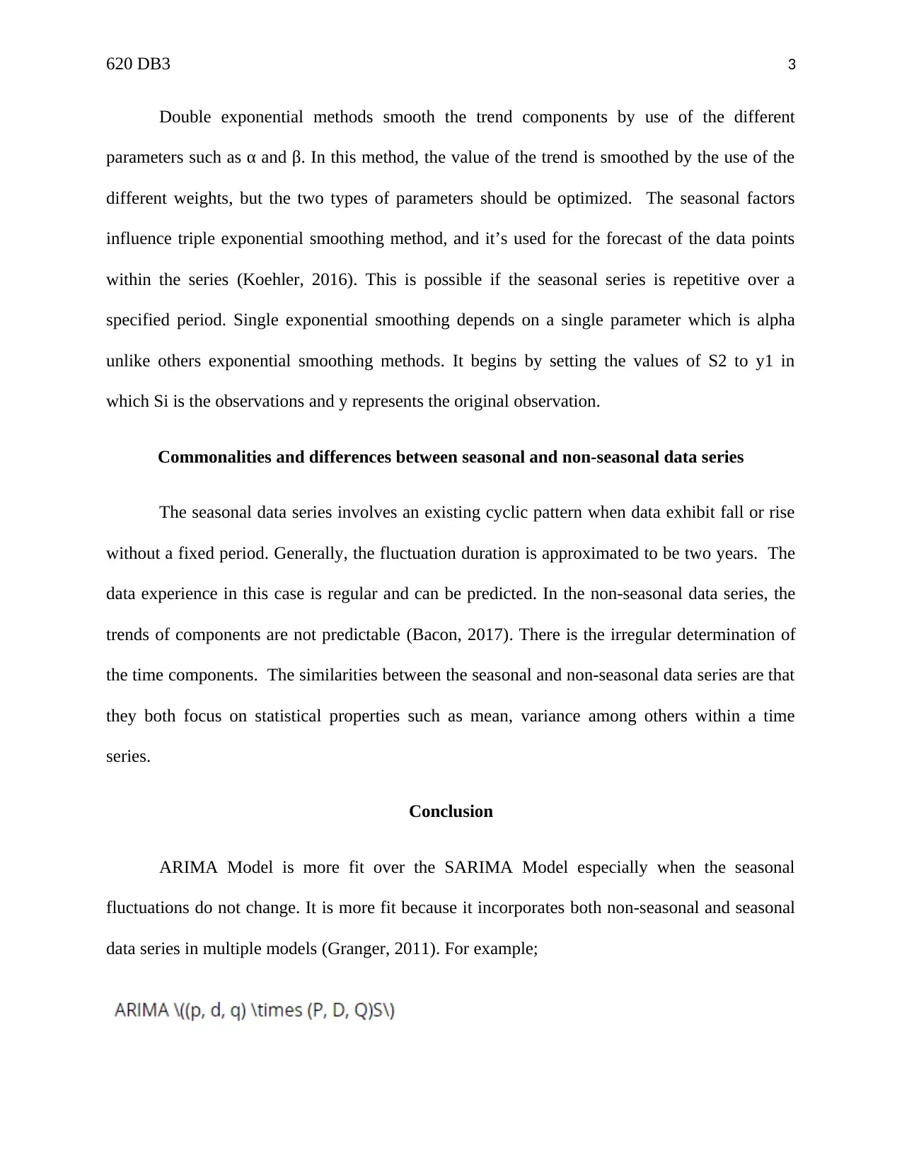
ARIMA Model is more fit over the SARIMA Model especially when the seasonal
fluctuations do not change. It is more fit because it incorporates both non-seasonal and seasonal
data series in multiple models (Granger, 2011). For example;

620 DB3 4
In this example, P represents the non-seasonal AR order while S represents the time series in
seasonal data series.

620 DB3 5
References
Bacon, D. W. (2017). Models For Forecasting Seasonal And Non-Seasonal Time Series (No. Tr-
118). Wisconsin Univ Madison Dept Of Statistics; Journal of forecasting, 18(5), 359-367.
Gardner Jr, E. S. (2015). Exponential smoothing: The state of the art. Journal of
forecasting, 4(1), 1-28.
Granger, C. W. (2011). Some properties of time series data and their use in econometric model
specification. Journal of econometrics, 16(1), 121-130.
Koehler, A. B. (2016). Exponential smoothing model selection for forecasting. International
journal of forecasting, 22(2), 239-247.