Project Evaluation and Analysis: ABC Ltd. Expansion Plant, Finance

This finance project analyzes the expansion plan of ABC Ltd., focusing on project evaluation. The assignment begins by calculating the initial outlay, considering building and equipment costs, and net working capital. It then proceeds to calculate operating cash flow over four years, factoring i...Read More

1
Finance

2
Table of Contents
Task 1(a)..........................................................................................................................................3
Calculation of initial outlay.........................................................................................................3
Calculation of operating cash flow..............................................................................................3
Calculation of terminal cash flow................................................................................................4
Calculation of NPV......................................................................................................................4
Task 1(b)..........................................................................................................................................5
Sensitivity analysis......................................................................................................................5
Scenario analysis.......................................................................................................................10
References......................................................................................................................................11

3
Task 1(a)
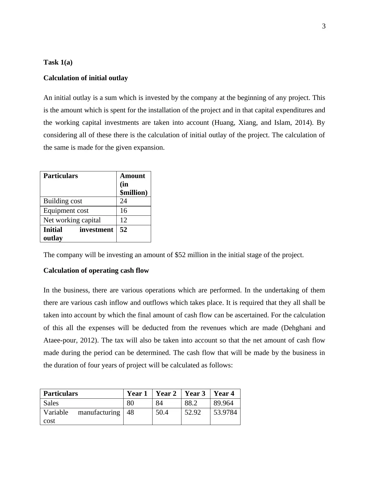
Calculation of initial outlay
An initial outlay is a sum which is invested by the company at the beginning of any project. This
is the amount which is spent for the installation of the project and in that capital expenditures and
the working capital investments are taken into account (Huang, Xiang, and Islam, 2014). By
considering all of these there is the calculation of initial outlay of the project. The calculation of
the same is made for the given expansion.
Particulars Amount
(in
$million)
Building cost 24
Equipment cost 16
Net working capital 12
Initial investment
outlay
52
The company will be investing an amount of $52 million in the initial stage of the project.
Calculation of operating cash flow
In the business, there are various operations which are performed. In the undertaking of them
there are various cash inflow and outflows which takes place. It is required that they all shall be
taken into account by which the final amount of cash flow can be ascertained. For the calculation
of this all the expenses will be deducted from the revenues which are made (Dehghani and
Ataee-pour, 2012). The tax will also be taken into account so that the net amount of cash flow
made during the period can be determined. The cash flow that will be made by the business in
the duration of four years of project will be calculated as follows:
Particulars Year 1 Year 2 Year 3 Year 4
Sales 80 84 88.2 89.964
Variable manufacturing
cost
48 50.4 52.92 53.9784

4
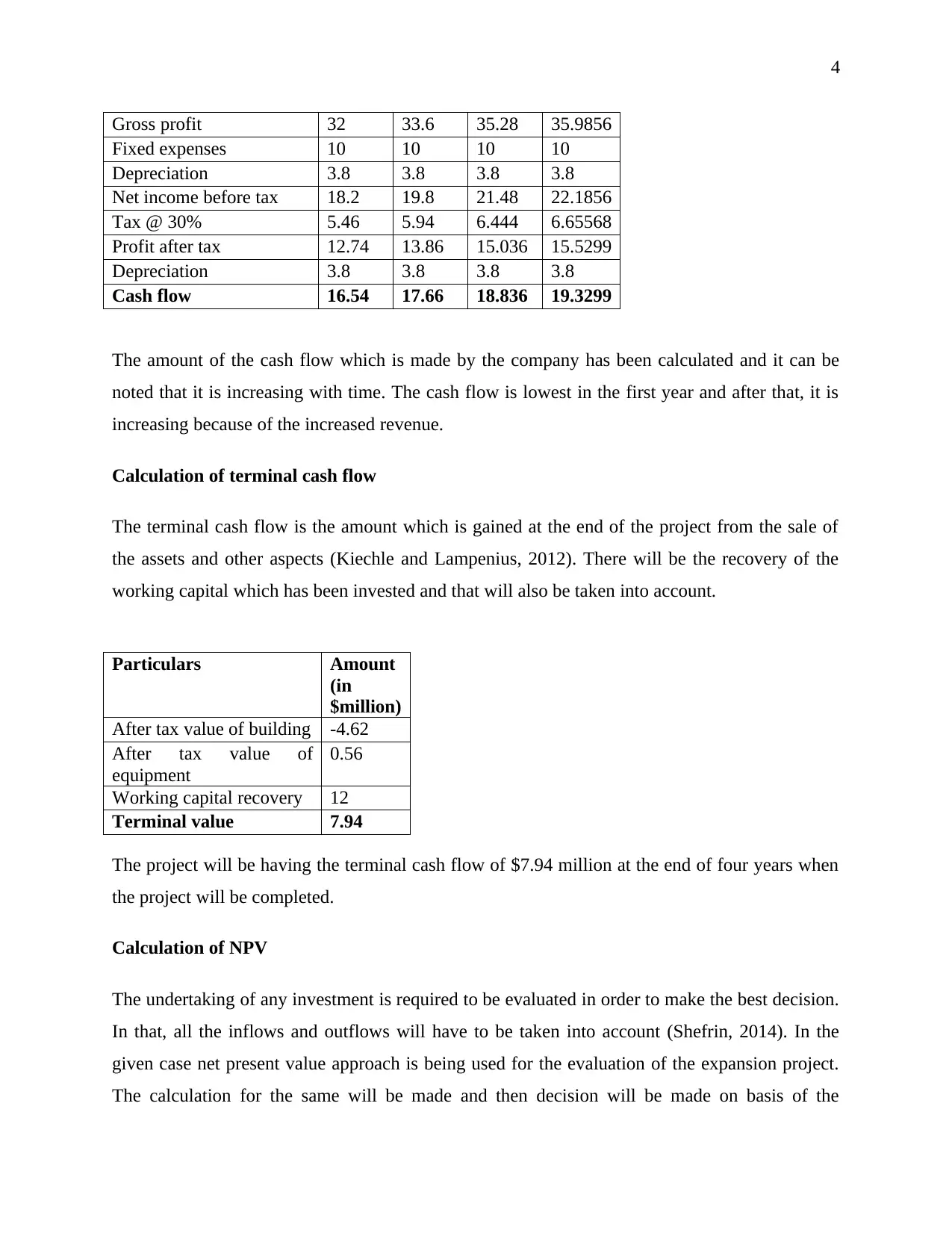
Gross profit 32 33.6 35.28 35.9856
Fixed expenses 10 10 10 10
Depreciation 3.8 3.8 3.8 3.8
Net income before tax 18.2 19.8 21.48 22.1856
Tax @ 30% 5.46 5.94 6.444 6.65568
Profit after tax 12.74 13.86 15.036 15.5299
Depreciation 3.8 3.8 3.8 3.8
Cash flow 16.54 17.66 18.836 19.3299
The amount of the cash flow which is made by the company has been calculated and it can be
noted that it is increasing with time. The cash flow is lowest in the first year and after that, it is
increasing because of the increased revenue.
Calculation of terminal cash flow
The terminal cash flow is the amount which is gained at the end of the project from the sale of
the assets and other aspects (Kiechle and Lampenius, 2012). There will be the recovery of the
working capital which has been invested and that will also be taken into account.
Particulars Amount
(in
$million)
After tax value of building -4.62
After tax value of
equipment
0.56
Working capital recovery 12
Terminal value 7.94
The project will be having the terminal cash flow of $7.94 million at the end of four years when
the project will be completed.
Calculation of NPV
The undertaking of any investment is required to be evaluated in order to make the best decision.
In that, all the inflows and outflows will have to be taken into account (Shefrin, 2014). In the
given case net present value approach is being used for the evaluation of the expansion project.
The calculation for the same will be made and then decision will be made on basis of the

5
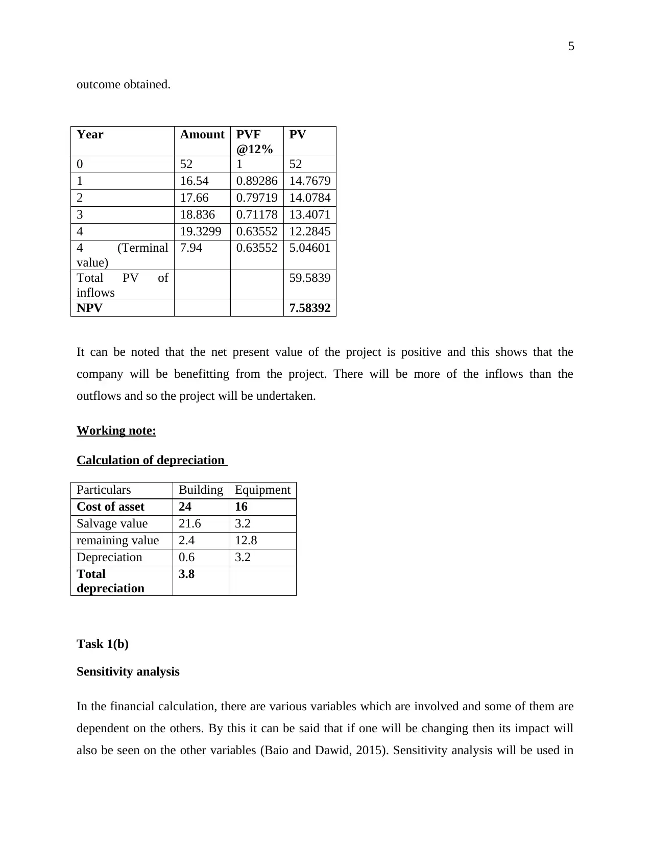
outcome obtained.
Year Amount PVF
@12%
PV
0 52 1 52
1 16.54 0.89286 14.7679
2 17.66 0.79719 14.0784
3 18.836 0.71178 13.4071
4 19.3299 0.63552 12.2845
4 (Terminal
value)
7.94 0.63552 5.04601
Total PV of
inflows
59.5839
NPV 7.58392
It can be noted that the net present value of the project is positive and this shows that the
company will be benefitting from the project. There will be more of the inflows than the
outflows and so the project will be undertaken.
Working note:
Calculation of depreciation
Particulars Building Equipment
Cost of asset 24 16
Salvage value 21.6 3.2
remaining value 2.4 12.8
Depreciation 0.6 3.2
Total
depreciation
3.8
Task 1(b)
Sensitivity analysis
In the financial calculation, there are various variables which are involved and some of them are
dependent on the others. By this it can be said that if one will be changing then its impact will
also be seen on the other variables (Baio and Dawid, 2015). Sensitivity analysis will be used in

6
such situations to analyze the variable which is most sensitive and will be affecting the outcome
the most.
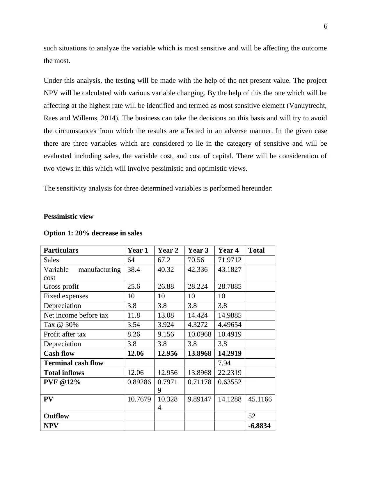
Under this analysis, the testing will be made with the help of the net present value. The project
NPV will be calculated with various variable changing. By the help of this the one which will be
affecting at the highest rate will be identified and termed as most sensitive element (Vanuytrecht,
Raes and Willems, 2014). The business can take the decisions on this basis and will try to avoid
the circumstances from which the results are affected in an adverse manner. In the given case
there are three variables which are considered to lie in the category of sensitive and will be
evaluated including sales, the variable cost, and cost of capital. There will be consideration of
two views in this which will involve pessimistic and optimistic views.
The sensitivity analysis for three determined variables is performed hereunder:
Pessimistic view
Option 1: 20% decrease in sales
Particulars Year 1 Year 2 Year 3 Year 4 Total
Sales 64 67.2 70.56 71.9712
Variable manufacturing
cost
38.4 40.32 42.336 43.1827
Gross profit 25.6 26.88 28.224 28.7885
Fixed expenses 10 10 10 10
Depreciation 3.8 3.8 3.8 3.8
Net income before tax 11.8 13.08 14.424 14.9885
Tax @ 30% 3.54 3.924 4.3272 4.49654
Profit after tax 8.26 9.156 10.0968 10.4919
Depreciation 3.8 3.8 3.8 3.8
Cash flow 12.06 12.956 13.8968 14.2919
Terminal cash flow 7.94
Total inflows 12.06 12.956 13.8968 22.2319
PVF @12% 0.89286 0.7971
9
0.71178 0.63552
PV 10.7679 10.328
4
9.89147 14.1288 45.1166
Outflow 52
NPV -6.8834

7
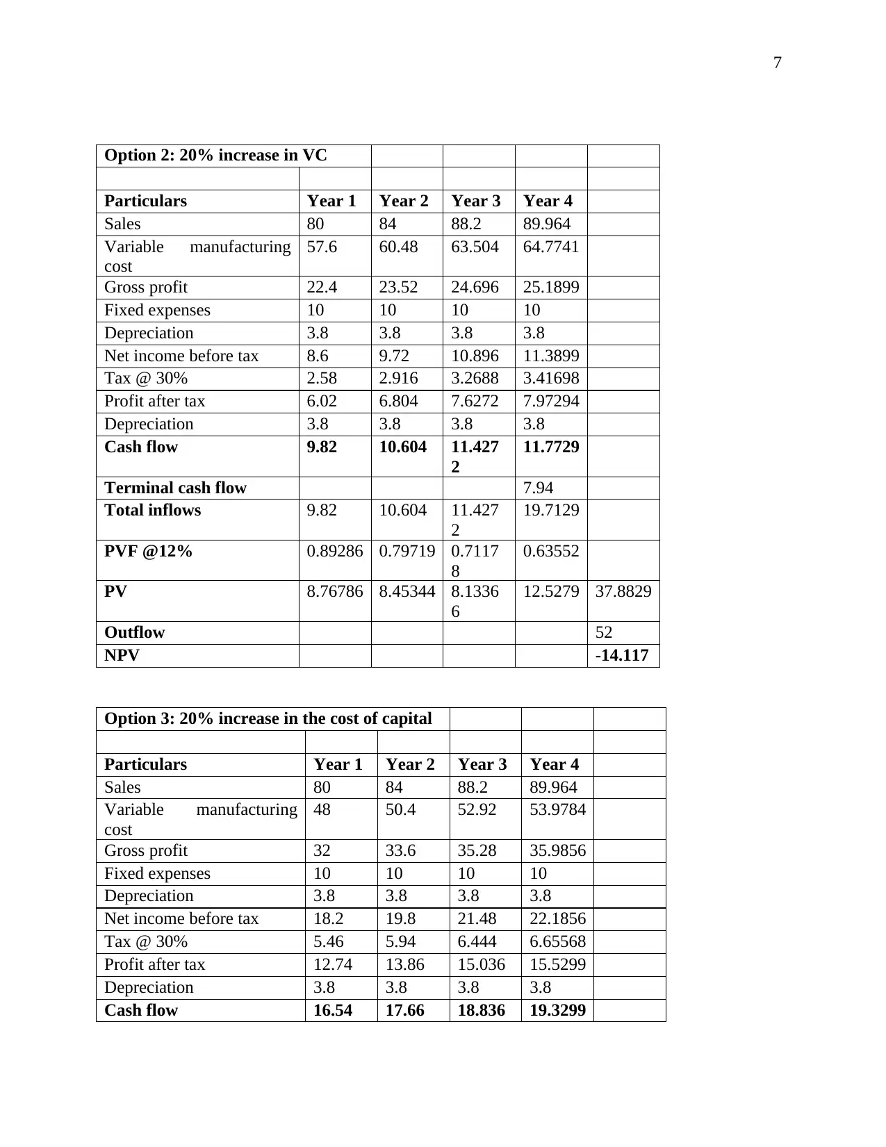
Option 2: 20% increase in VC
Particulars Year 1 Year 2 Year 3 Year 4
Sales 80 84 88.2 89.964
Variable manufacturing
cost
57.6 60.48 63.504 64.7741
Gross profit 22.4 23.52 24.696 25.1899
Fixed expenses 10 10 10 10
Depreciation 3.8 3.8 3.8 3.8
Net income before tax 8.6 9.72 10.896 11.3899
Tax @ 30% 2.58 2.916 3.2688 3.41698
Profit after tax 6.02 6.804 7.6272 7.97294
Depreciation 3.8 3.8 3.8 3.8
Cash flow 9.82 10.604 11.427
2
11.7729
Terminal cash flow 7.94
Total inflows 9.82 10.604 11.427
2
19.7129
PVF @12% 0.89286 0.79719 0.7117
8
0.63552
PV 8.76786 8.45344 8.1336
6
12.5279 37.8829
Outflow 52
NPV -14.117
Option 3: 20% increase in the cost of capital
Particulars Year 1 Year 2 Year 3 Year 4
Sales 80 84 88.2 89.964
Variable manufacturing
cost
48 50.4 52.92 53.9784
Gross profit 32 33.6 35.28 35.9856
Fixed expenses 10 10 10 10
Depreciation 3.8 3.8 3.8 3.8
Net income before tax 18.2 19.8 21.48 22.1856
Tax @ 30% 5.46 5.94 6.444 6.65568
Profit after tax 12.74 13.86 15.036 15.5299
Depreciation 3.8 3.8 3.8 3.8
Cash flow 16.54 17.66 18.836 19.3299

8
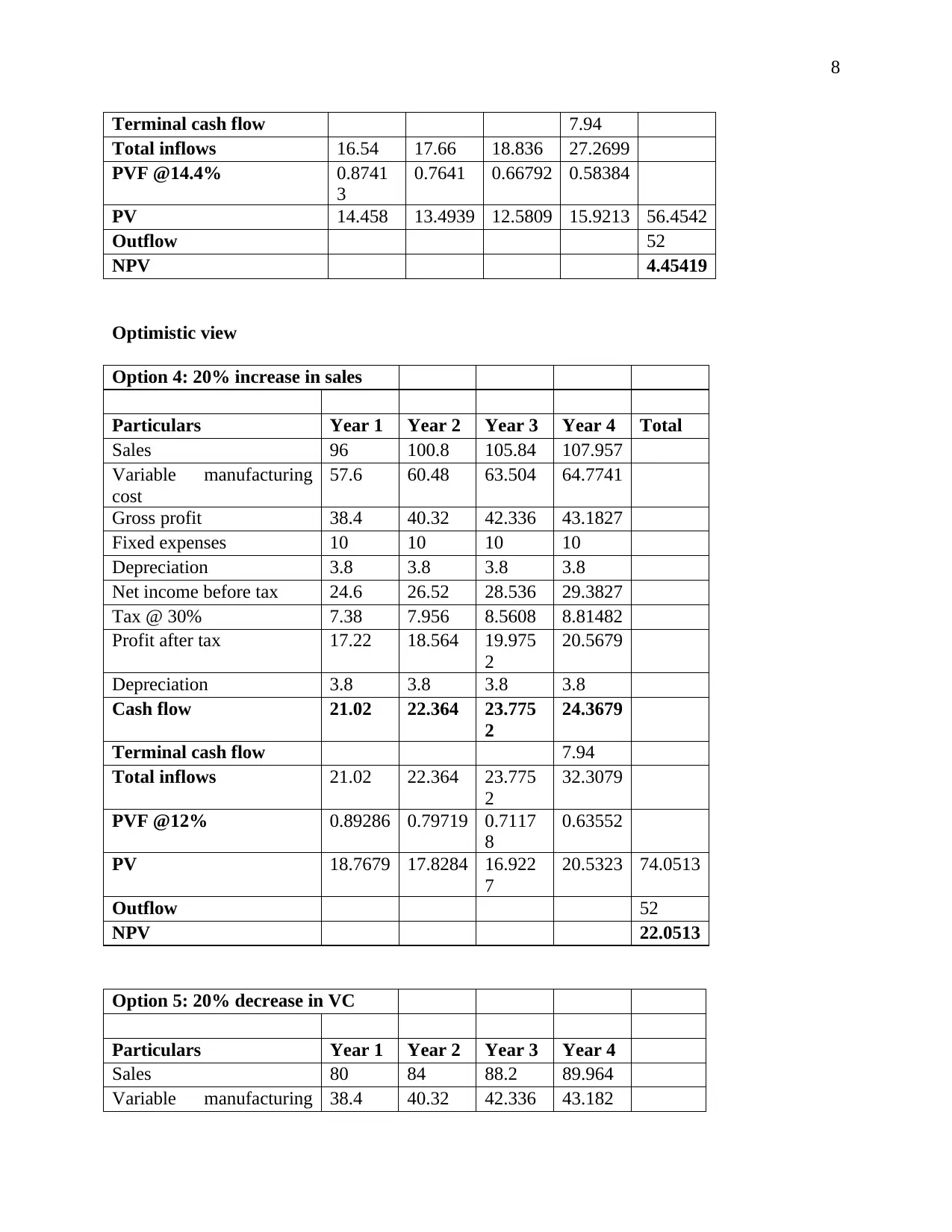
Terminal cash flow 7.94
Total inflows 16.54 17.66 18.836 27.2699
PVF @14.4% 0.8741
3
0.7641 0.66792 0.58384
PV 14.458 13.4939 12.5809 15.9213 56.4542
Outflow 52
NPV 4.45419
Optimistic view
Option 4: 20% increase in sales
Particulars Year 1 Year 2 Year 3 Year 4 Total
Sales 96 100.8 105.84 107.957
Variable manufacturing
cost
57.6 60.48 63.504 64.7741
Gross profit 38.4 40.32 42.336 43.1827
Fixed expenses 10 10 10 10
Depreciation 3.8 3.8 3.8 3.8
Net income before tax 24.6 26.52 28.536 29.3827
Tax @ 30% 7.38 7.956 8.5608 8.81482
Profit after tax 17.22 18.564 19.975
2
20.5679
Depreciation 3.8 3.8 3.8 3.8
Cash flow 21.02 22.364 23.775
2
24.3679
Terminal cash flow 7.94
Total inflows 21.02 22.364 23.775
2
32.3079
PVF @12% 0.89286 0.79719 0.7117
8
0.63552
PV 18.7679 17.8284 16.922
7
20.5323 74.0513
Outflow 52
NPV 22.0513
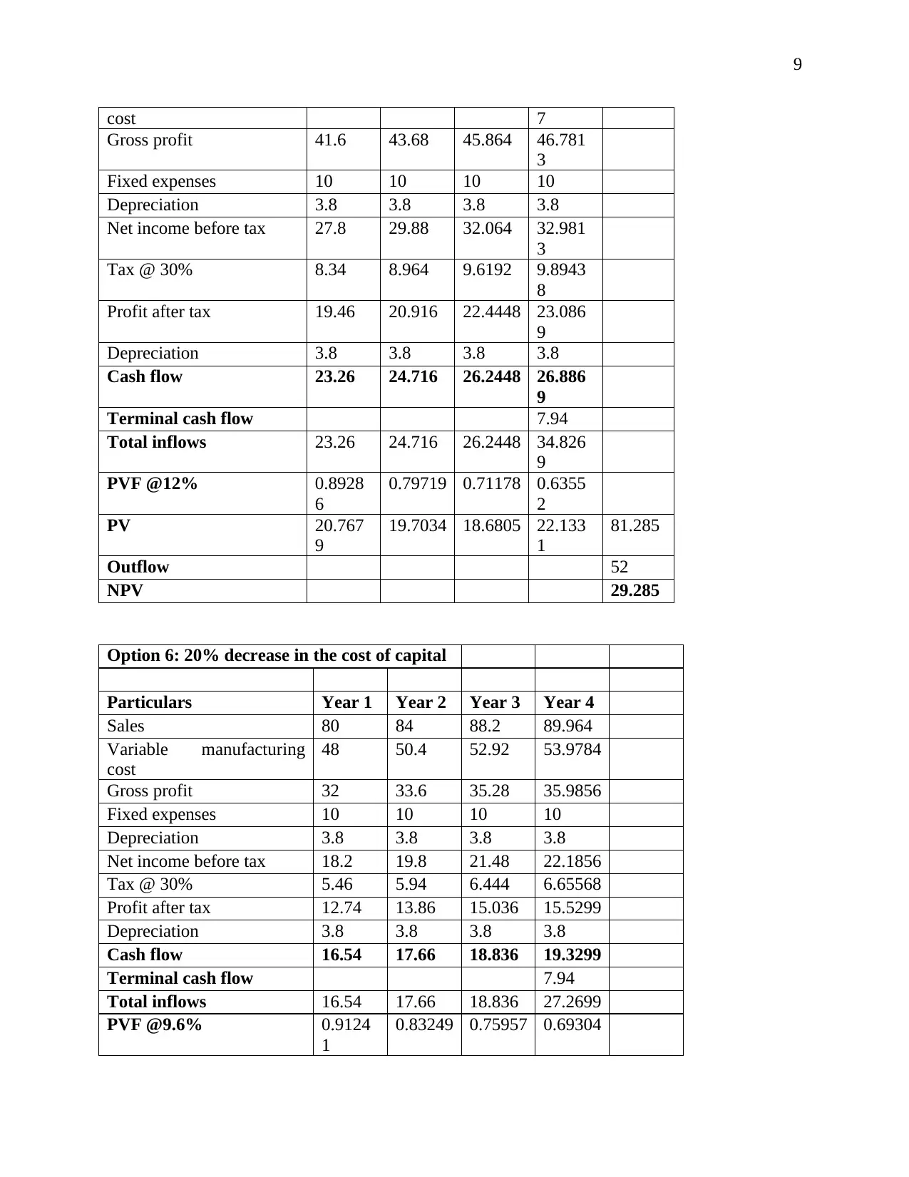
Option 5: 20% decrease in VC
Particulars Year 1 Year 2 Year 3 Year 4
Sales 80 84 88.2 89.964
Variable manufacturing 38.4 40.32 42.336 43.182

9
cost 7
Gross profit 41.6 43.68 45.864 46.781
3
Fixed expenses 10 10 10 10
Depreciation 3.8 3.8 3.8 3.8
Net income before tax 27.8 29.88 32.064 32.981
3
Tax @ 30% 8.34 8.964 9.6192 9.8943
8
Profit after tax 19.46 20.916 22.4448 23.086
9
Depreciation 3.8 3.8 3.8 3.8
Cash flow 23.26 24.716 26.2448 26.886
9
Terminal cash flow 7.94
Total inflows 23.26 24.716 26.2448 34.826
9
PVF @12% 0.8928
6
0.79719 0.71178 0.6355
2
PV 20.767
9
19.7034 18.6805 22.133
1
81.285
Outflow 52
NPV 29.285
Option 6: 20% decrease in the cost of capital
Particulars Year 1 Year 2 Year 3 Year 4
Sales 80 84 88.2 89.964
Variable manufacturing
cost
48 50.4 52.92 53.9784
Gross profit 32 33.6 35.28 35.9856
Fixed expenses 10 10 10 10
Depreciation 3.8 3.8 3.8 3.8
Net income before tax 18.2 19.8 21.48 22.1856
Tax @ 30% 5.46 5.94 6.444 6.65568
Profit after tax 12.74 13.86 15.036 15.5299
Depreciation 3.8 3.8 3.8 3.8
Cash flow 16.54 17.66 18.836 19.3299
Terminal cash flow 7.94
Total inflows 16.54 17.66 18.836 27.2699
PVF @9.6% 0.9124
1
0.83249 0.75957 0.69304

10
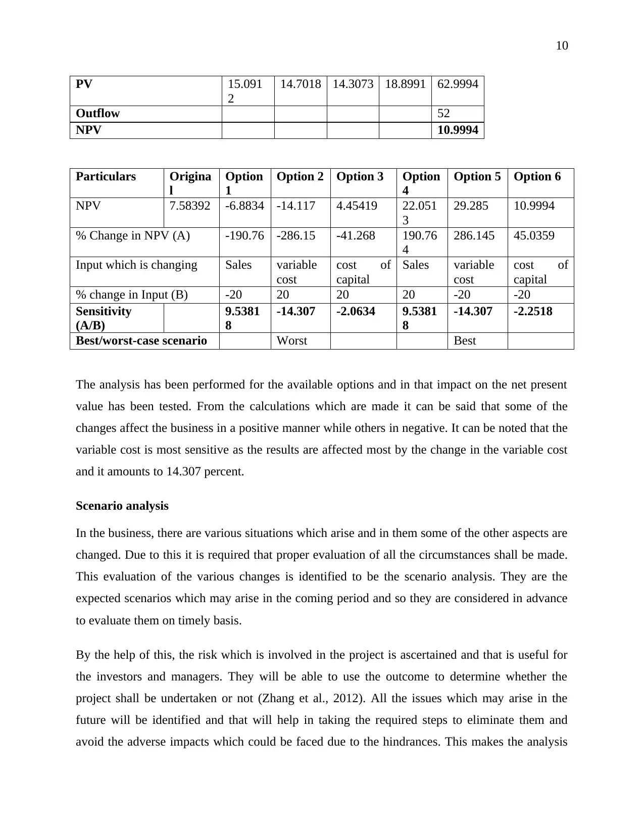
PV 15.091
2
14.7018 14.3073 18.8991 62.9994
Outflow 52
NPV 10.9994
Particulars Origina
l
Option
1
Option 2 Option 3 Option
4
Option 5 Option 6
NPV 7.58392 -6.8834 -14.117 4.45419 22.051
3
29.285 10.9994
% Change in NPV (A) -190.76 -286.15 -41.268 190.76
4
286.145 45.0359
Input which is changing Sales variable
cost
cost of
capital
Sales variable
cost
cost of
capital
% change in Input (B) -20 20 20 20 -20 -20
Sensitivity
(A/B)
9.5381
8
-14.307 -2.0634 9.5381
8
-14.307 -2.2518
Best/worst-case scenario Worst Best
The analysis has been performed for the available options and in that impact on the net present
value has been tested. From the calculations which are made it can be said that some of the
changes affect the business in a positive manner while others in negative. It can be noted that the
variable cost is most sensitive as the results are affected most by the change in the variable cost
and it amounts to 14.307 percent.
Scenario analysis
In the business, there are various situations which arise and in them some of the other aspects are
changed. Due to this it is required that proper evaluation of all the circumstances shall be made.
This evaluation of the various changes is identified to be the scenario analysis. They are the
expected scenarios which may arise in the coming period and so they are considered in advance
to evaluate them on timely basis.
By the help of this, the risk which is involved in the project is ascertained and that is useful for
the investors and managers. They will be able to use the outcome to determine whether the
project shall be undertaken or not (Zhang et al., 2012). All the issues which may arise in the
future will be identified and that will help in taking the required steps to eliminate them and
avoid the adverse impacts which could be faced due to the hindrances. This makes the analysis

11
useful and in this best-case and worst-case scenarios are identified. From the calculations which
are made above it can be noted that option 2 with increase in the variable cost by 20% is the
worst case as the net present value in such case will be negative. The decrease in the variable
cost by 20% has been made and with that highest amount of NPV is made possible. Due to this it
will be considered as the best-case scenario.

12
References
Baio, G. and Dawid, A.P. (2015) Probabilistic sensitivity analysis in health
economics. Statistical methods in medical research, 24(6), pp.615-634.
Dehghani, H. and Ataee-pour, M. (2012) Determination of the effect of operating cost
uncertainty on mining project evaluation. Resources Policy, 37(1), pp.109-117.
Huang, X., Xiang, L. and Islam, S.M. (2014) Optimal project adjustment and
selection. Economic Modelling, 36, pp.391-397.
Kiechle, D. and Lampenius, N. (2012) The Terminal Value and Inflation Controversy. Journal of
Applied Corporate Finance, 24(3), pp.101-107.
Shefrin, H. (2014) Free cash Flow, Valuation and Growth Opportunities Bias. Journal of
Investment Management, 12(4), pp.4-26.
Vanuytrecht, E., Raes, D. and Willems, P. (2014) Global sensitivity analysis of yield output from
the water productivity model. Environmental Modelling & Software, 51, pp.323-332.
Zhang, Q., Ishihara, K.N., Mclellan, B.C. and Tezuka, T. (2012) Scenario analysis on future
electricity supply and demand in Japan. Energy, 38(1), pp.376-385.