Assignment: Accounting Decision Support Tools - [Date] - Finance

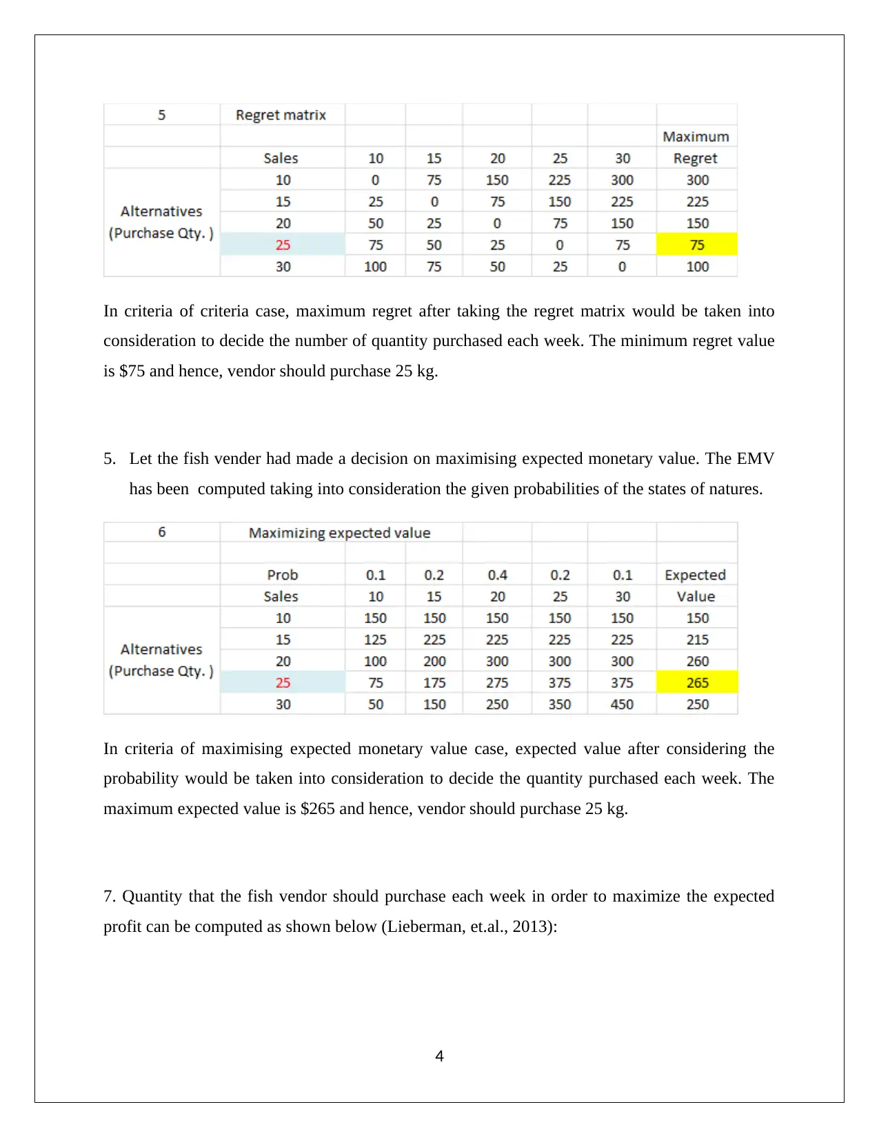
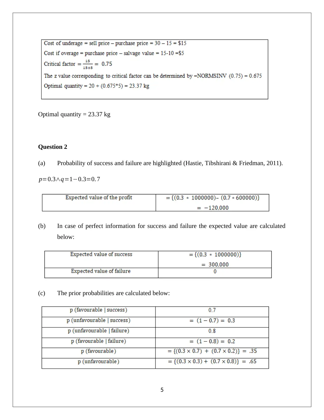
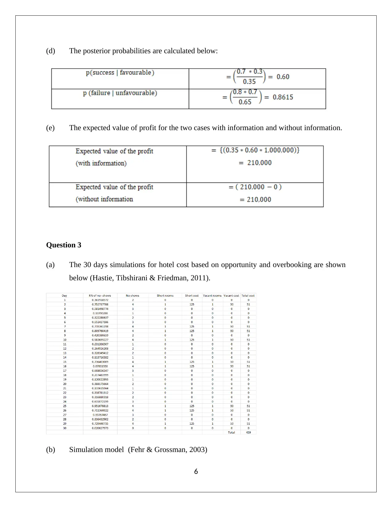
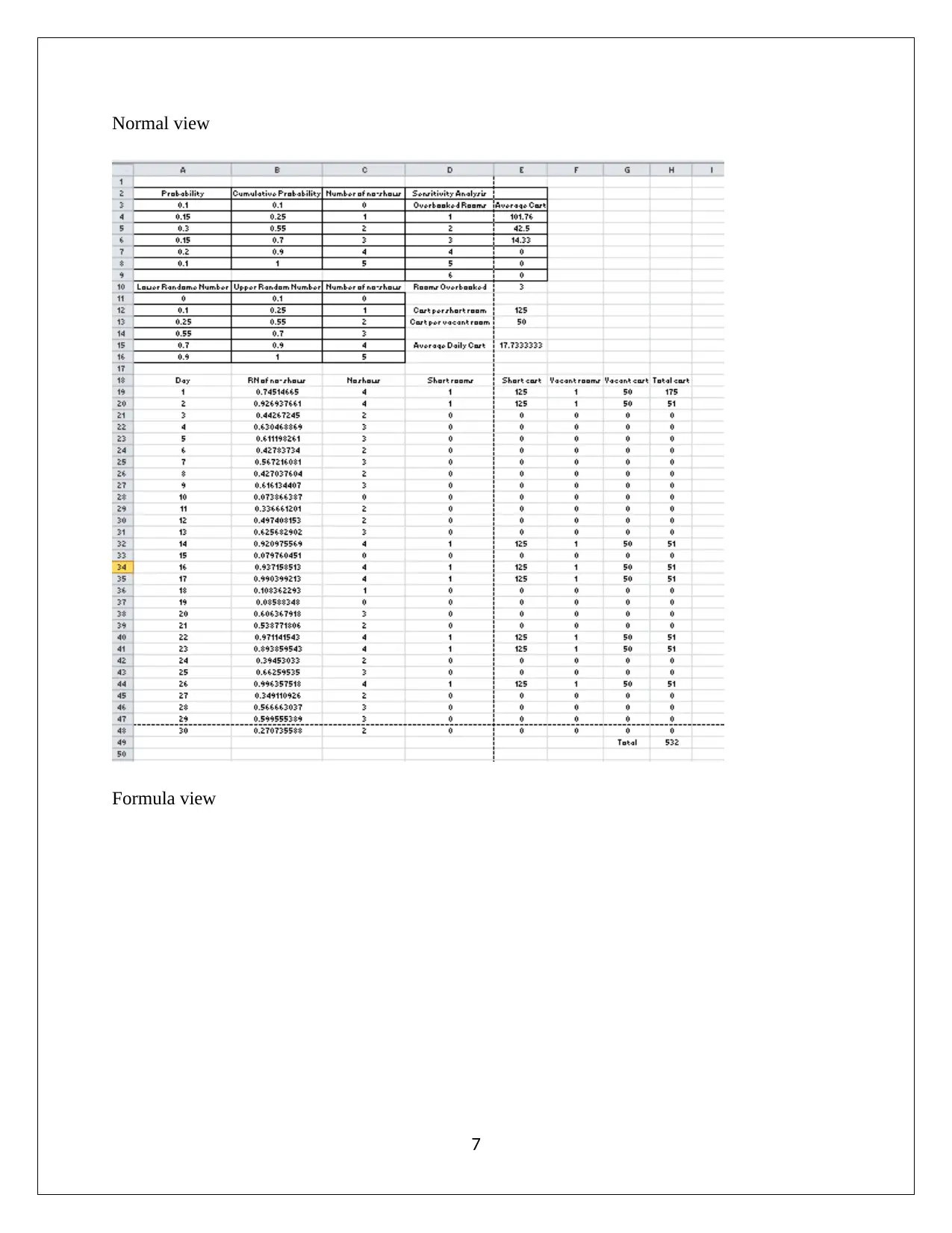
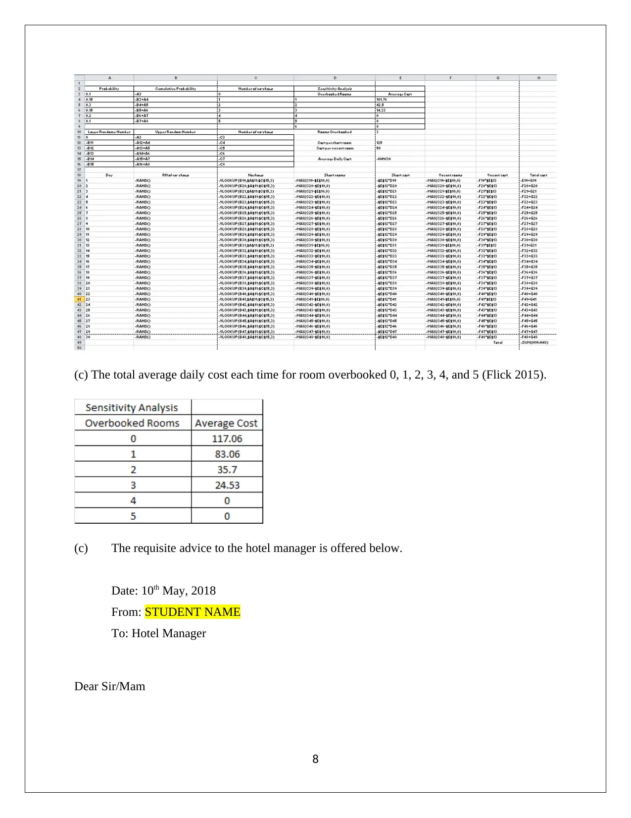
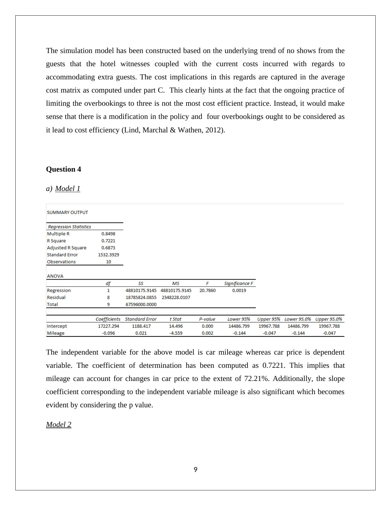
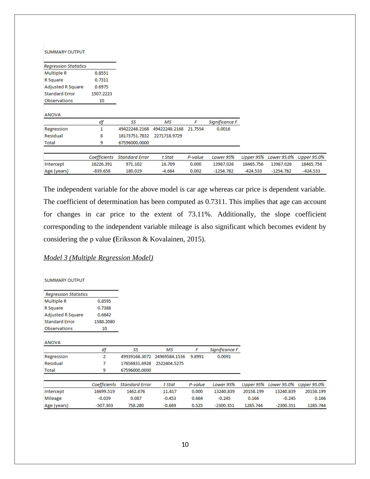
This assignment provides a comprehensive analysis of accounting decision support tools, covering various aspects of financial decision-making. It begins with an exploration of the decision-making process, including the use of payoff matrices and different decision criteria such as optimist, pessimist, Laplace, and regret criteria, and maximizing expected monetary value. The assignment then delves into probability analysis, calculating prior and posterior probabilities, and evaluating the expected value of profit with and without information. Further, it includes simulation models for hotel cost analysis based on opportunity and overbooking, providing recommendations to hotel managers. The assignment also covers regression analysis, comparing different models to predict car prices based on mileage and age, and finally, it explores breakeven analysis and profit maximization for a manufacturer producing multiple products. The solutions provided offer practical insights and applications of these tools in financial decision-making.

Accounting Decision Support Tools
Assignment item 3
[Pick the date]
Student Name

Question 1
(a) The following steps are involved in the decision making process (Hair, et. al., 2015).
 There are certain set of expectations from a decision which need to be defined from
the outset and also the requsiite outcomes need identification.
 The alternatives that are possible for the decision maker need to be highlighted.
 Each alternative need to be individually analysed thereby identifying the likely
outcomes along with their underlying probability.
 The various outcomes and their underlying risk need to represented in the form of a
payoff matrix.
 The decision making model needs to be applied taking into cognizance the payoff
matrix to reach approrpaite decision.
(b) The decision maker has various strategies that can be implemented given a particular
decision and these are classified as alternatives. Also, there are possible future scenarios
which are beyond the decision maker’s control and are termed as states of nature. The
alternatives and state of nature tend to be linked since for a given state of nature, a particular
alternative may be found suitable. However, given the underlying risk, an alternative needs to
be chosen considering the likelihood of the future states of nature (Hair, et. al., 2015).
(c) Sales records are highlighted below:
1

1. Conditional profits matrix is as exhibited below based on the input data provided
(Lieberman, et.al., 2013):
1. Let the fish vendor be an optimist. The respective payoff matrix is indicated below.
In optimist case, maximum payoff would be taken into consideration to decide the number of
quantity purchased each week. The maximum value is $450 and hence, vendor should purchase
30kg.
2. Let the fish vendor be an pessimist. The respective payoff matrix is indicated below.
2

In pessimist case, maximum payoff after taking the minimum value would be taken into
consideration to decide the number of quantity purchased each week. The maximum value of all
minimum values is $150 and hence, vendor should purchase 10kg.
3. Let the fish vender had used Laplace criteria. The respective payoff matrix is indicated
below.
In Laplace criteria case, maximum payoff after taking the average value would be taken into
consideration to decide the number of quantity purchased each week. In order to take average, t
has been assumed that the probability of each state of nature is the same or 0.2. The maximum
value is $255 and hence, vendor should purchase 25 kg.
4. Let the fish vender had used criteria of regret. The respective regret matrix is indicated
below.
3

In criteria of criteria case, maximum regret after taking the regret matrix would be taken into
consideration to decide the number of quantity purchased each week. The minimum regret value
is $75 and hence, vendor should purchase 25 kg.
5. Let the fish vender had made a decision on maximising expected monetary value. The EMV
has been computed taking into consideration the given probabilities of the states of natures.
In criteria of maximising expected monetary value case, expected value after considering the
probability would be taken into consideration to decide the quantity purchased each week. The
maximum expected value is $265 and hence, vendor should purchase 25 kg.
7. Quantity that the fish vendor should purchase each week in order to maximize the expected
profit can be computed as shown below (Lieberman, et.al., 2013):
4

Optimal quantity = 23.37 kg
Question 2
(a) Probability of success and failure are highlighted (Hastie, Tibshirani & Friedman, 2011).
p=0.3∧q=1−0.3=0. 7
(b) In case of perfect information for success and failure the expected value are calculated
below:
(c) The prior probabilities are calculated below:
5

(d) The posterior probabilities are calculated below:
(e) The expected value of profit for the two cases with information and without information.
Question 3
(a) The 30 days simulations for hotel cost based on opportunity and overbooking are shown
below (Hastie, Tibshirani & Friedman, 2011).
(b) Simulation model (Fehr & Grossman, 2003)
6

Normal view
Formula view
7

(c) The total average daily cost each time for room overbooked 0, 1, 2, 3, 4, and 5 (Flick 2015).
(c) The requisite advice to the hotel manager is offered below.
Date: 10th May, 2018
From: STUDENT NAME
To: Hotel Manager
Dear Sir/Mam
8

The simulation model has been constructed based on the underlying trend of no shows from the
guests that the hotel witnesses coupled with the current costs incurred with regards to
accommodating extra guests. The cost implications in this regards are captured in the average
cost matrix as computed under part C. This clearly hints at the fact that the ongoing practice of
limiting the overbookings to three is not the most cost efficient practice. Instead, it would make
sense that there is a modification in the policy and four overbookings ought to be considered as
it lead to cost efficiency (Lind, Marchal & Wathen, 2012).
Question 4
a) Model 1
The independent variable for the above model is car mileage whereas car price is dependent
variable. The coefficient of determination has been computed as 0.7221. This implies that
mileage can account for changes in car price to the extent of 72.21%. Additionally, the slope
coefficient corresponding to the independent variable mileage is also significant which becomes
evident by considering the p value.
Model 2
9

The independent variable for the above model is car age whereas car price is dependent variable.
The coefficient of determination has been computed as 0.7311. This implies that age can account
for changes in car price to the extent of 73.11%. Additionally, the slope coefficient
corresponding to the independent variable mileage is also significant which becomes evident by
considering the p value (Eriksson & Kovalainen, 2015).
Model 3 (Multiple Regression Model)
10

The independent variables for the above model are car age and car mileage whereas car price is
dependent variable. The coefficient of determination has been computed as 0.7388. This implies
that age and mileage can on a joint basis account for changes in car price to the extent of
73.88%. However, the two slope coefficient corresponding to the two independent variables i.e,
mileage and age are not significant which becomes evident by considering the p value (Lind,
Marchal & Wathen, 2012).
Best Choice
From this choice, there is instant rejection of Model 3 owing to the insignificance of the slope
coefficients. Between the two simple regression models, Model 2 (Age- Dependent Variable)
would be a preferred choice owing to higher coefficient of determination and higher significance
of the slope coefficient.
b) As discussed above, owing to higher ability to predict accurately, Model 2 would be
preferred over Model 1 as far as the two simple regression models are concerned. The
negative slope coefficient value of age is not surprising since it would be expected that a
higher depreciation would be charged as age of the car increases and also the model gets
outdated. Besides, the slope coefficient pertaining to mileage on expected pattern is negative
considering the increasing wear and tear to the car and the components owing to the higher
mileage (Medhi, 2001).
c) In relation to model 3, a rather confusing observation from the output is that despite the
coefficient of determination being close to 0.75, neither of the independent variables have a
statistically significant slope coefficient even at 10% significance level. This aberration can be
accounted for by the high correlation between the two given independent variables. This is
clearly unacceptable considering that multiple regression assumes that the correlation between
independent variables is negligible (Taylor & Cihon, 2004). Thus, Model 3 should be ignored
and must not be put to use.
11

Question 5
(a) Manufacturer makes product A
Selling price of product A= $15
Variable cost per unit of product A = $7
Fixed cost of product A =$2400
“At breakeven the profit would be zero (Fehr & Grossman, 2003) .”
12

Therefore, the number of units of A sold to breakeven would be 300.
(b) Desired Profit = $1600
13

Therefore, the number of units of A required would be 500 for the before tax profit of $1600.
(c) One more product B is added for manufacturing.
Selling price of product B = $20
Variable cost per unit of product B = $10
Fixe cost of product B =$3600
Manufacturer has decided to product A: B = 2: 1
14

Hence, the units of A = 2000 and B = 1000.
15

References
Eriksson, P. & Kovalainen, A. (2015). Quantitative methods in business research (3rd ed.).
London: Sage Publications.
Fehr, F. H., & Grossman, G. (2003). An introduction to sets, probability and hypothesis testing
(3rd ed.). Ohio: Heath.
Flick, U. (2015). Introducing research methodology: A beginner's guide to doing a research
project (4th ed.). New York: Sage Publications.
Hair, J. F., Wolfinbarger, M., Money, A. H., Samouel, P., & Page, M. J. (2015). Essentials of
business research methods (2nd ed.). New York: Routledge.
Harmon, M. (2011). Hypothesis Testing in Excel - The Excel Statistical Master (7th ed.). Florida:
Mark Harmon.
Hastie, T., Tibshirani, R. & Friedman, J. (2011). The Elements of Statistical Learning (4th
ed.). New York: Springer Publications.
Hillier, F. (2006). Introduction to Operations Research. (6th ed.). New York: McGraw Hill
Publications.
Lieberman, F. J., Nag, B., Hiller, F.S. & Basu, P. (2013). Introduction To Operations Research
(5th ed.). New Delhi: Tata McGraw Hill Publishers.
Lind, A.D., Marchal, G.W. & Wathen, A.S. (2012). Statistical Techniques in Business and
Economics (15th ed.). New York : McGraw-Hill/Irwin.
Medhi, J. (2001). Statistical Methods: An Introductory Text (4th ed.). Sydney: New Age
International.
Taylor, K. J. & Cihon, C. (2004). Statistical Techniques for Data Analysis (2nd ed.). Melbourne:
CRC Press.
16