Comprehensive Accounting and Finance Analysis: University Assignment
VerifiedAdded on 2023/01/18
|15
|3369
|27
Homework Assignment
AI Summary
This finance assignment delves into various aspects of accounting and finance. It begins with a calculation of the amount needed for a future sum, considering monthly compounding interest rates. The assignment then evaluates a project's financial viability using net present value and analyzes cash flows. It proceeds to assess the value of financial assets, including superannuation funds and share portfolios, and calculates monthly pension amounts. Furthermore, the assignment explores real interest rates, negative gearing, and their implications. It also covers investment risk, dividend imputation, and the calculation of monthly and annual returns for BHP Ltd, considering both Australian and international shareholders. The solution provides detailed calculations and explanations of the financial concepts involved.

Running head: ACCOUNTING AND FINANCE
Accounting and Finance
Name of the Student:
Name of the University:
Author’s Note:
Accounting and Finance
Name of the Student:
Name of the University:
Author’s Note:
Paraphrase This Document
Need a fresh take? Get an instant paraphrase of this document with our AI Paraphraser

1ACCOUNTING AND FINANCE
Table of Contents
Question 1..................................................................................................................................2
Question 2..................................................................................................................................6
Question 3..................................................................................................................................7
References................................................................................................................................14
2ACCOUNTING AND FINANCE
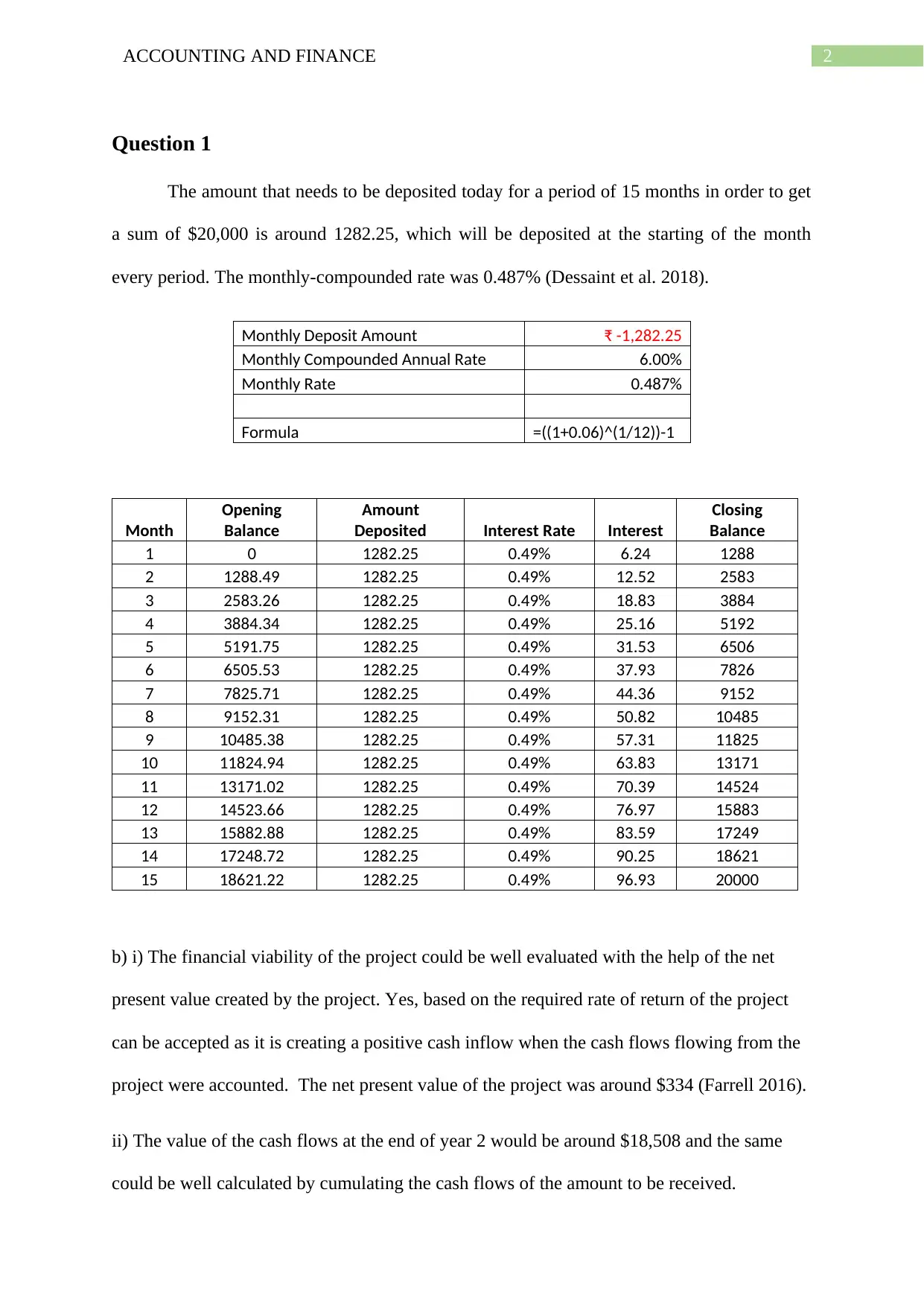
Question 1
The amount that needs to be deposited today for a period of 15 months in order to get
a sum of $20,000 is around 1282.25, which will be deposited at the starting of the month
every period. The monthly-compounded rate was 0.487% (Dessaint et al. 2018).
Monthly Deposit Amount ₹ -1,282.25
Monthly Compounded Annual Rate 6.00%
Monthly Rate 0.487%
Formula =((1+0.06)^(1/12))-1
Month
Opening
Balance
Amount
Deposited Interest Rate Interest
Closing
Balance
1 0 1282.25 0.49% 6.24 1288
2 1288.49 1282.25 0.49% 12.52 2583
3 2583.26 1282.25 0.49% 18.83 3884
4 3884.34 1282.25 0.49% 25.16 5192
5 5191.75 1282.25 0.49% 31.53 6506
6 6505.53 1282.25 0.49% 37.93 7826
7 7825.71 1282.25 0.49% 44.36 9152
8 9152.31 1282.25 0.49% 50.82 10485
9 10485.38 1282.25 0.49% 57.31 11825
10 11824.94 1282.25 0.49% 63.83 13171
11 13171.02 1282.25 0.49% 70.39 14524
12 14523.66 1282.25 0.49% 76.97 15883
13 15882.88 1282.25 0.49% 83.59 17249
14 17248.72 1282.25 0.49% 90.25 18621
15 18621.22 1282.25 0.49% 96.93 20000
b) i) The financial viability of the project could be well evaluated with the help of the net
present value created by the project. Yes, based on the required rate of return of the project
can be accepted as it is creating a positive cash inflow when the cash flows flowing from the
project were accounted. The net present value of the project was around $334 (Farrell 2016).
ii) The value of the cash flows at the end of year 2 would be around $18,508 and the same
could be well calculated by cumulating the cash flows of the amount to be received.
⊘ This is a preview!⊘
Do you want full access?
Subscribe today to unlock all pages.
Trusted by 1+ million students worldwide
3ACCOUNTING AND FINANCE
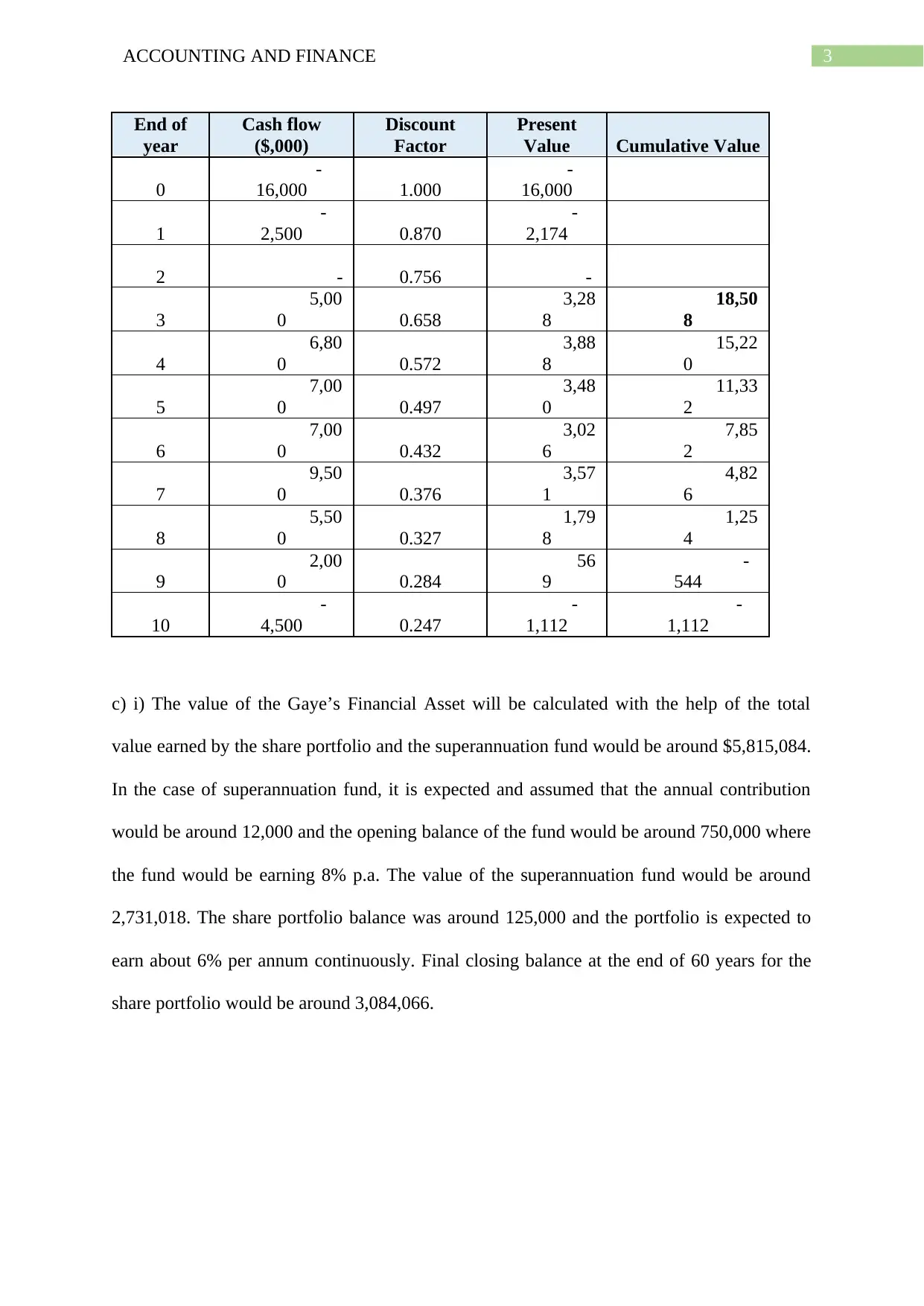
End of
year
Cash flow
($,000)
Discount
Factor
Present
Value Cumulative Value
0
-
16,000 1.000
-
16,000
1
-
2,500 0.870
-
2,174
2 - 0.756 -
3
5,00
0 0.658
3,28
8
18,50
8
4
6,80
0 0.572
3,88
8
15,22
0
5
7,00
0 0.497
3,48
0
11,33
2
6
7,00
0 0.432
3,02
6
7,85
2
7
9,50
0 0.376
3,57
1
4,82
6
8
5,50
0 0.327
1,79
8
1,25
4
9
2,00
0 0.284
56
9
-
544
10
-
4,500 0.247
-
1,112
-
1,112
c) i) The value of the Gaye’s Financial Asset will be calculated with the help of the total
value earned by the share portfolio and the superannuation fund would be around $5,815,084.
In the case of superannuation fund, it is expected and assumed that the annual contribution
would be around 12,000 and the opening balance of the fund would be around 750,000 where
the fund would be earning 8% p.a. The value of the superannuation fund would be around
2,731,018. The share portfolio balance was around 125,000 and the portfolio is expected to
earn about 6% per annum continuously. Final closing balance at the end of 60 years for the
share portfolio would be around 3,084,066.
Paraphrase This Document
Need a fresh take? Get an instant paraphrase of this document with our AI Paraphraser
4ACCOUNTING AND FINANCE
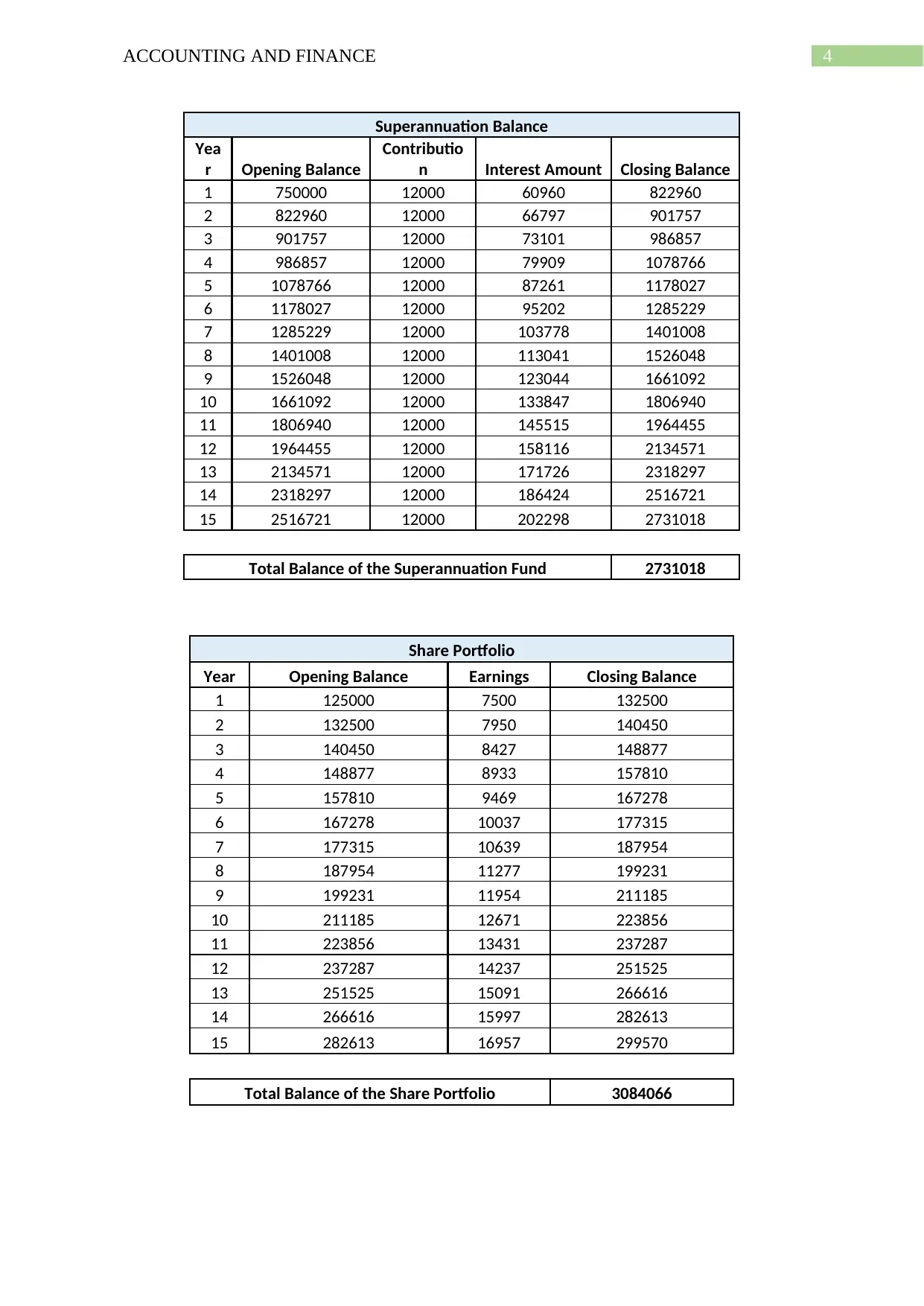
Superannuation Balance
Yea
r Opening Balance
Contributio
n Interest Amount Closing Balance
1 750000 12000 60960 822960
2 822960 12000 66797 901757
3 901757 12000 73101 986857
4 986857 12000 79909 1078766
5 1078766 12000 87261 1178027
6 1178027 12000 95202 1285229
7 1285229 12000 103778 1401008
8 1401008 12000 113041 1526048
9 1526048 12000 123044 1661092
10 1661092 12000 133847 1806940
11 1806940 12000 145515 1964455
12 1964455 12000 158116 2134571
13 2134571 12000 171726 2318297
14 2318297 12000 186424 2516721
15 2516721 12000 202298 2731018
Total Balance of the Superannuation Fund 2731018
Share Portfolio
Year Opening Balance Earnings Closing Balance
1 125000 7500 132500
2 132500 7950 140450
3 140450 8427 148877
4 148877 8933 157810
5 157810 9469 167278
6 167278 10037 177315
7 177315 10639 187954
8 187954 11277 199231
9 199231 11954 211185
10 211185 12671 223856
11 223856 13431 237287
12 237287 14237 251525
13 251525 15091 266616
14 266616 15997 282613
15 282613 16957 299570
Total Balance of the Share Portfolio 3084066
5ACCOUNTING AND FINANCE
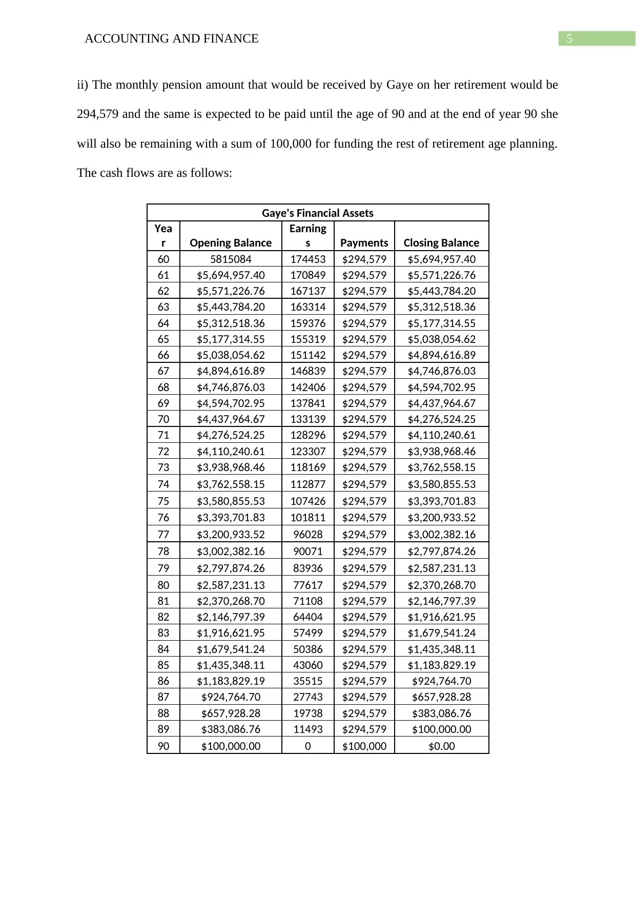
ii) The monthly pension amount that would be received by Gaye on her retirement would be
294,579 and the same is expected to be paid until the age of 90 and at the end of year 90 she
will also be remaining with a sum of 100,000 for funding the rest of retirement age planning.
The cash flows are as follows:
Gaye's Financial Assets
Yea
r Opening Balance
Earning
s Payments Closing Balance
60 5815084 174453 $294,579 $5,694,957.40
61 $5,694,957.40 170849 $294,579 $5,571,226.76
62 $5,571,226.76 167137 $294,579 $5,443,784.20
63 $5,443,784.20 163314 $294,579 $5,312,518.36
64 $5,312,518.36 159376 $294,579 $5,177,314.55
65 $5,177,314.55 155319 $294,579 $5,038,054.62
66 $5,038,054.62 151142 $294,579 $4,894,616.89
67 $4,894,616.89 146839 $294,579 $4,746,876.03
68 $4,746,876.03 142406 $294,579 $4,594,702.95
69 $4,594,702.95 137841 $294,579 $4,437,964.67
70 $4,437,964.67 133139 $294,579 $4,276,524.25
71 $4,276,524.25 128296 $294,579 $4,110,240.61
72 $4,110,240.61 123307 $294,579 $3,938,968.46
73 $3,938,968.46 118169 $294,579 $3,762,558.15
74 $3,762,558.15 112877 $294,579 $3,580,855.53
75 $3,580,855.53 107426 $294,579 $3,393,701.83
76 $3,393,701.83 101811 $294,579 $3,200,933.52
77 $3,200,933.52 96028 $294,579 $3,002,382.16
78 $3,002,382.16 90071 $294,579 $2,797,874.26
79 $2,797,874.26 83936 $294,579 $2,587,231.13
80 $2,587,231.13 77617 $294,579 $2,370,268.70
81 $2,370,268.70 71108 $294,579 $2,146,797.39
82 $2,146,797.39 64404 $294,579 $1,916,621.95
83 $1,916,621.95 57499 $294,579 $1,679,541.24
84 $1,679,541.24 50386 $294,579 $1,435,348.11
85 $1,435,348.11 43060 $294,579 $1,183,829.19
86 $1,183,829.19 35515 $294,579 $924,764.70
87 $924,764.70 27743 $294,579 $657,928.28
88 $657,928.28 19738 $294,579 $383,086.76
89 $383,086.76 11493 $294,579 $100,000.00
90 $100,000.00 0 $100,000 $0.00
⊘ This is a preview!⊘
Do you want full access?
Subscribe today to unlock all pages.
Trusted by 1+ million students worldwide
6ACCOUNTING AND FINANCE
Question 2
i) The real rate of interest is the type of interest rate an investor saver or the lender
expects to receive after considering the inflation factor into account. Real Interest
rate is calculated as Nominal Interest Rate- Inflation Rate or the expected
percentage of inflation rate. The importance of the real interest rate can be well
seen if in a given economy the level of inflation is about 5%, which might be too
high. However, if the prevailing interest rate is to be about 7% then there are
chances that the investors can still protect their money. Thus, the difference can be
well observed with the help of the given scenario. The client would be receiving
the annual real rate of interest from the investment, which is around 0.5% on the
sum of $100,000. If considering the factor for the real rate of interest, if the
interest rate increases then the client would be compensated in the form of higher
return (Hung, 2016).
ii) Negative gearing is the phenomenon where one borrows money and invests it in
income generating assets but the returns form the assets is less than the
repayments and the outgoings on those assets. One of the key advantage of the
negative gearing is that the losses are adjusted against all the other incomes that
reduces the total taxable income and hence the tax payable is reduced. The
wealthy Australians are using this concept in order to reduce their tax burdens and
thus they are getting an opportunity to inflate the house prices (Blunden, 2016).
The people having a stable income purchase houses by taking loan and they let it
to the other people. The rents that are charged might not meet the mortgage
amount of the loan. This would help them subsidise their taxable amount.
Negative gearing has become a deliberate investment strategy at present. The
wealthy people are intentionally running a house property at an operating loss.
Paraphrase This Document
Need a fresh take? Get an instant paraphrase of this document with our AI Paraphraser
7ACCOUNTING AND FINANCE
They are therefore being able to build an asset portfolio with the minimum efforts
and it would become cash positive in the long run. The practice of the negative
gearing has inflated the house prices in Australia every year. The investors used to
take loans from the bank by telling lies, generally termed as the liar loans (Cho, Li
& Uren 2017). This has reduced the faith of the customers on the Australian banks
as well. The risks involved in this concept have awakened the economy and there
has been changes in the Labour’s Policy, which is reducing the prices of the house
at present and making it affordable for the commoners of the country.
Question 3
i) Risk is a part of investment with which an investor gets an exposure of investing
and gathering return from a specified assets class. Risk and return are the key
integral part of an investment. Risk in terms of investment or the investment risk
shows the probability or the likelihood reflecting a percentage of loss relative to
the return earned by the investor (Muda & Hasibuan, 2018). No risk is not a bad
thing in-fact some risk is good when viewed from the context of portfolio
management. However, risk is solely determined by the characteristics of the asset
class in which the investor is invested. Every Financial instruments have some or
other kind of risk, investor wants compensation in the form of higher return for
higher risk taken. However, it is crucial to note that the risk and return of an
individual may vary depending on the financial goals and investment plans. It is
required the return to risk ratio should be optimally higher where the investor can
earn a high amount of investment profit from the same (García, 2017).
ii) Dividend Imputation or Franking Credit is a type of tax credit allowing the
Companies operating in the Australia to pass on the tax credit to the shareholders
of the company. Franking Credits or the Dividend imputation removes the effect
8ACCOUNTING AND FINANCE
of double taxation where taxation would not be charged at both the shareholder’s
and the investor’s level. The Australian Franking Credit would only be applicable
to the Australian Resident where they will be getting avoidance of double taxation
from the benefit of franking credits. The nonresident of Australia at the base case
would be applicable for a 30% of withholding tax on un-franked dividend.
However, if the resident resides in a tax treaty country than the effective tax rate
could come down to around 15% and may come to 0% depending on the profile of
the investors (Shrivastav, 2017). In the case of foreign investor, there would be
some restriction in getting or usage of the franking credit but on the other hand,
the domestic shareholders can easily use the franking credit for reducing the
effective tax rate of the company. Franking credit can be categorically divided
into three steps based on the release and identification of the same:
Immediate franking credits: Credits that will be received when the
company will pay the dividend.
Stockpiled franking credits: Planned Structured credits, which would be
given in special cases like share buyback and special dividends paid by the
company.
Future franking credits: The credit would be paid in future via the future
tax payments paid.
iii) The 2018 monthly return for the BHP Ltd Company was as follows:
BHP Ltd Company (BHP)
Date Open Close
Dividends
((100%
Franked)
Adjusted
Closing
Price
Monthly
Returns
(%)
Return
in
Amount
($)
Jan 29.57 30.2 30.20 100
Feb 30.2 30.5 30.50 1% 101.0
Mar 30.5 28.21 0.705852 28.92 -8% 93.4
Apr 28.21 30.95 30.95 10% 102.5
⊘ This is a preview!⊘
Do you want full access?
Subscribe today to unlock all pages.
Trusted by 1+ million students worldwide
9ACCOUNTING AND FINANCE
May 30.95 32.79 32.79 6% 108.6
Jun 32.79 33.91 33.91 3% 112.3
Jul 33.91 34.86 34.86 3% 115.4
Aug 34.86 33.21 33.21 -5% 110.0
Sep 33.21 34.63 0.855978 35.49 4% 114.7
Oct 34.63 32.21 32.21 -7% 106.7
Nov 32.21 30.69 30.69 -5% 101.6
Dec 30.69 34.23 34.23 12% 113.3
iv) The average monthly return for the BHP was around 1.34%.
v) The annual holding period return (in both $ and % terms) for an international
(non-Australian) shareholder of BH is around 12.96% and the same has been done
after taking into account the 30% tax-rate. In terms of $ value they would be
earning around $113.3 + ((0.7058+0.8559)*(1-tax rate of 30%)), which is around
114.4.
vi) The annual holding period return for an Australian Resident shareholders of BHP
would be around 18.52% as the dividends would be fully franked and on a post-
tax basis the Australian Investor would be enjoying a higher effective economic
benefits. On a basis of dollar value the Australian Resident would be earning a
sum of $114.9 where the net investment was around $100.
vii) The monthly returns (%) for the Australian share market (MKT) during 2018 are
as follows:
Australian All Ordinaries Index (MKT)
Date Open Close Return
(%)
Return
in
Amount
($)
Jan 6146.5 6117.3 100
Feb 6117.3 5868.9 -4.1% 95.9
Mar 5868.9 6071.6 3.5% 99.3
Apr 6071.6 6123.5 0.9% 100.1
May 6123.5 6289.7 2.7% 102.8
Jun 6289.7 6366.2 1.2% 104.1
Jul 6366.2 6427.8 1.0% 105.1
Paraphrase This Document
Need a fresh take? Get an instant paraphrase of this document with our AI Paraphraser
10ACCOUNTING AND FINANCE
Aug 6427.8 6325.5 -1.6% 103.4
Sep 6325.5 5913.3 -6.5% 96.7
Oct 5913.3 5749.3 -2.8% 94.0
Nov 5749.3 5709.4 -0.7% 93.3
Dec 5709.4 5783.3 1.3% 94.5
Annual Holding Period Return -5.46%
Average Monthly Return -0.47%
Standard Deviation 3.02%
viii) The average monthly return (%) for the MKT (ALL ORDS) was around -0.47%.
ix) The annual holding period return (in % terms) for the Australian share market
(MKT) during 2018 was around -5.46%.
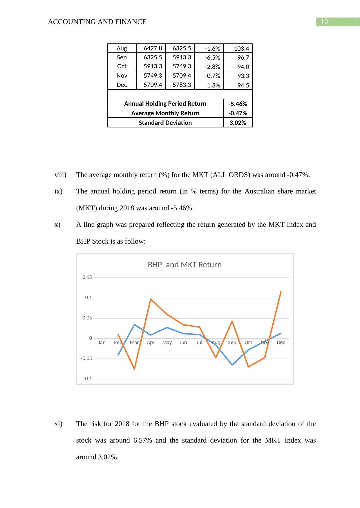
x) A line graph was prepared reflecting the return generated by the MKT Index and
BHP Stock is as follow:
Jan Feb Mar Apr May Jun Jul Aug Sep Oct Nov Dec
-0.1
-0.05
0
0.05
0.1
0.15
BHP and MKT Return
xi) The risk for 2018 for the BHP stock evaluated by the standard deviation of the
stock was around 6.57% and the standard deviation for the MKT Index was
around 3.02%.
Aug 6427.8 6325.5 -1.6% 103.4
Sep 6325.5 5913.3 -6.5% 96.7
Oct 5913.3 5749.3 -2.8% 94.0
Nov 5749.3 5709.4 -0.7% 93.3
Dec 5709.4 5783.3 1.3% 94.5
Annual Holding Period Return -5.46%
Average Monthly Return -0.47%
Standard Deviation 3.02%
viii) The average monthly return (%) for the MKT (ALL ORDS) was around -0.47%.
ix) The annual holding period return (in % terms) for the Australian share market
(MKT) during 2018 was around -5.46%.
x) A line graph was prepared reflecting the return generated by the MKT Index and
BHP Stock is as follow:
Jan Feb Mar Apr May Jun Jul Aug Sep Oct Nov Dec
-0.1
-0.05
0
0.05
0.1
0.15
BHP and MKT Return
xi) The risk for 2018 for the BHP stock evaluated by the standard deviation of the
stock was around 6.57% and the standard deviation for the MKT Index was
around 3.02%.
11ACCOUNTING AND FINANCE
xii) Beta shows the sensitivity or the movement of the stock with represent to a
benchmark index say MKT Index. A BETA of 1.12 reflects that when market
changes by 1% the stock is expected to move by around 1.12% reflecting the
sensitivity of the stock. Higher beta stock reflects higher volatility stocks where
the value of the stocks can change rapidly with the change in the benchmark
index. It is generally considered that stock whose beta are less than 1.0 are
considered to be more safer in terms of volatility and sensitivity than those above
these level. A beta of 1.12 reflects that the stock is indeed somewhat risky when
benchmarked with the market index. Beta is an important component, which is
used by an investors and analysts for determine the required return on equity for
share via the capital asset pricing model.
xiii) The required return for the BHP Ltd Company’s Stock was around 10.42% and
the same has been calculated with the help of the formula:
CAPM= (Risk Free Rate of Return (Rf) + (Return on Market-Risk Free Rate of
Return)*Beta.
Capital Asset Pricing Model (CAPM)
R (e) = R(F)+Beta*R(m)-R(f)
Risk Free Rate of Return 2.29%
Return on Market 9.55%
Beta 1.12
CAPM (Re) 10.42%
xiv) The security market line was drawn by taking the risk free rate of return, return on
market and the beta of the stock and the following graph was prepared:
⊘ This is a preview!⊘
Do you want full access?
Subscribe today to unlock all pages.
Trusted by 1+ million students worldwide
1 out of 15
Related Documents


Your All-in-One AI-Powered Toolkit for Academic Success.
+13062052269
info@desklib.com
Available 24*7 on WhatsApp / Email
![[object Object]](/_next/static/media/star-bottom.7253800d.svg)
Unlock your academic potential
Copyright © 2020–2026 A2Z Services. All Rights Reserved. Developed and managed by ZUCOL.