Design and Performance Analysis of ROF System in Optical Network

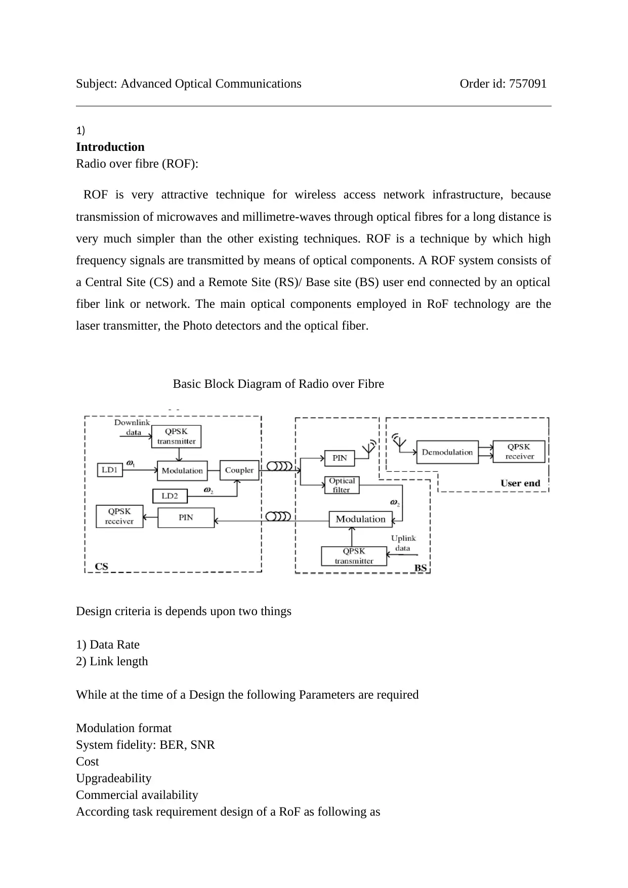
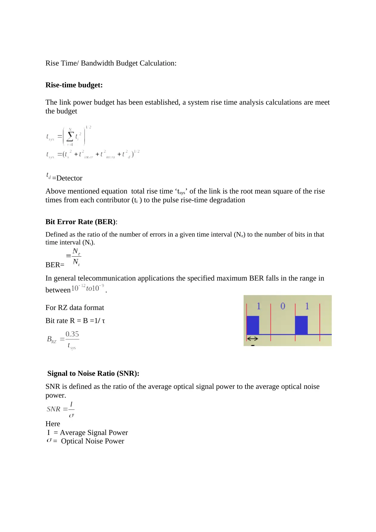
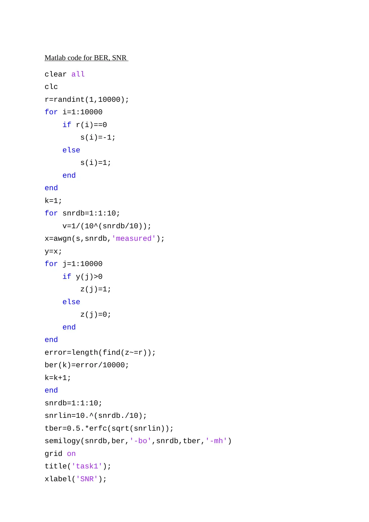
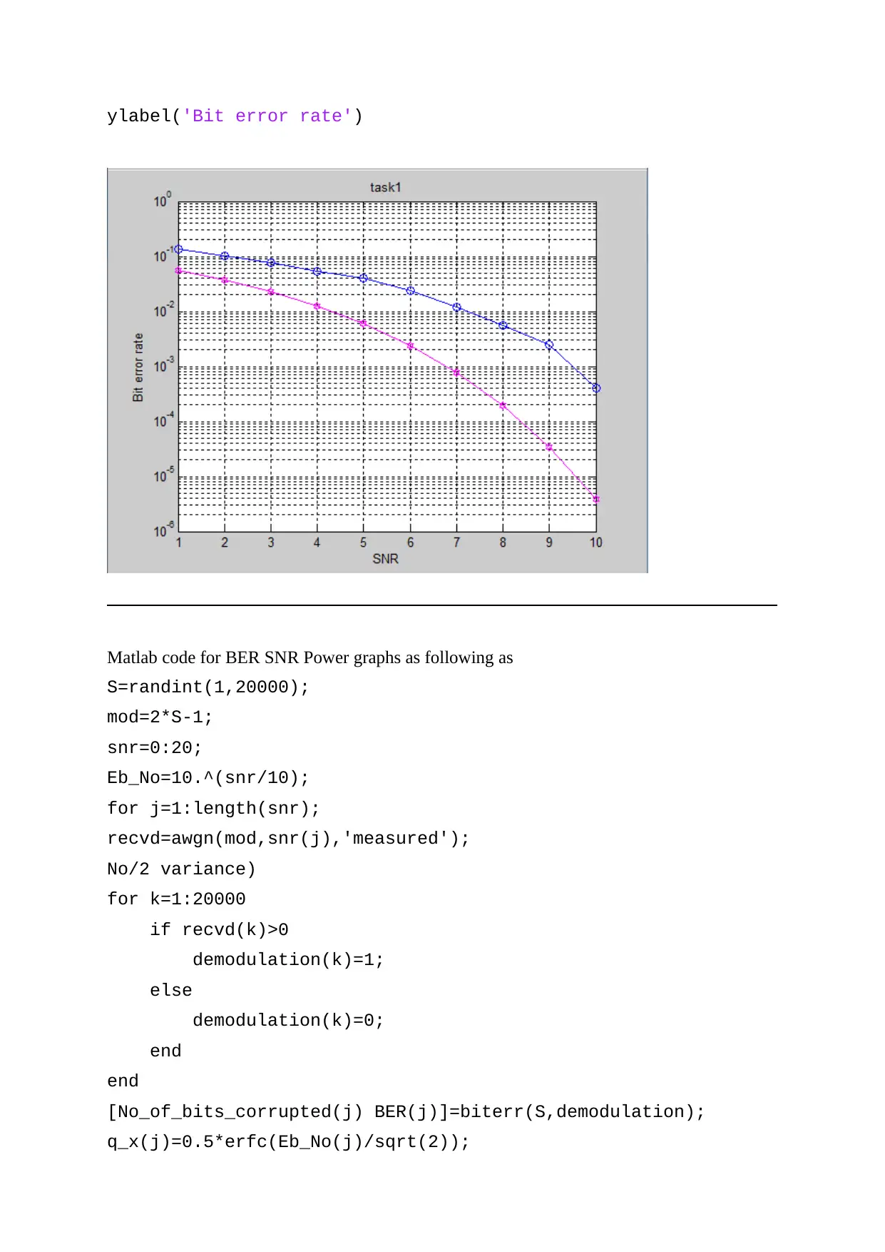
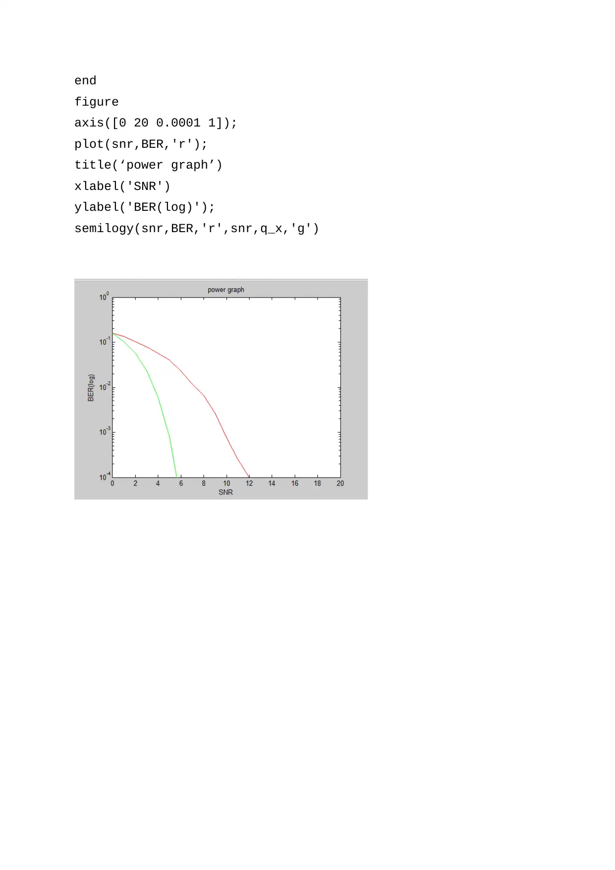
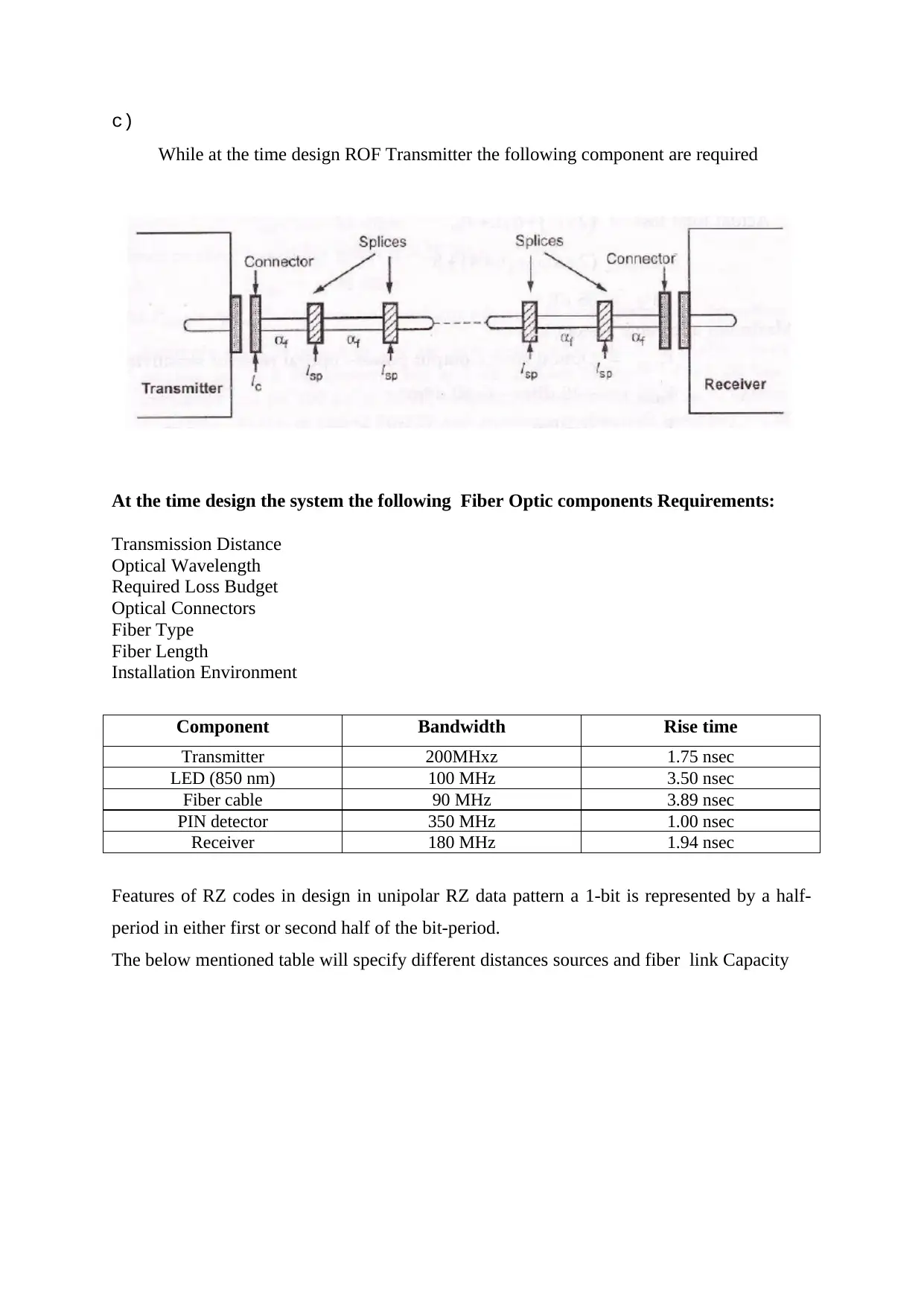
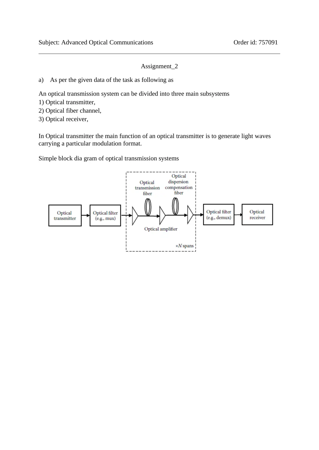
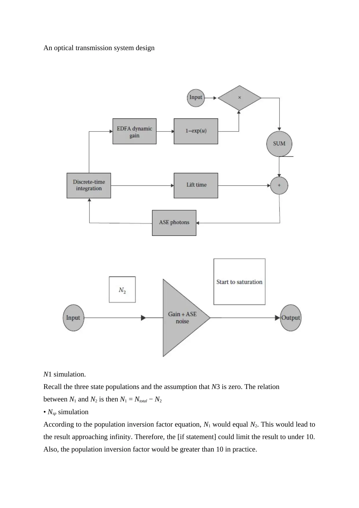
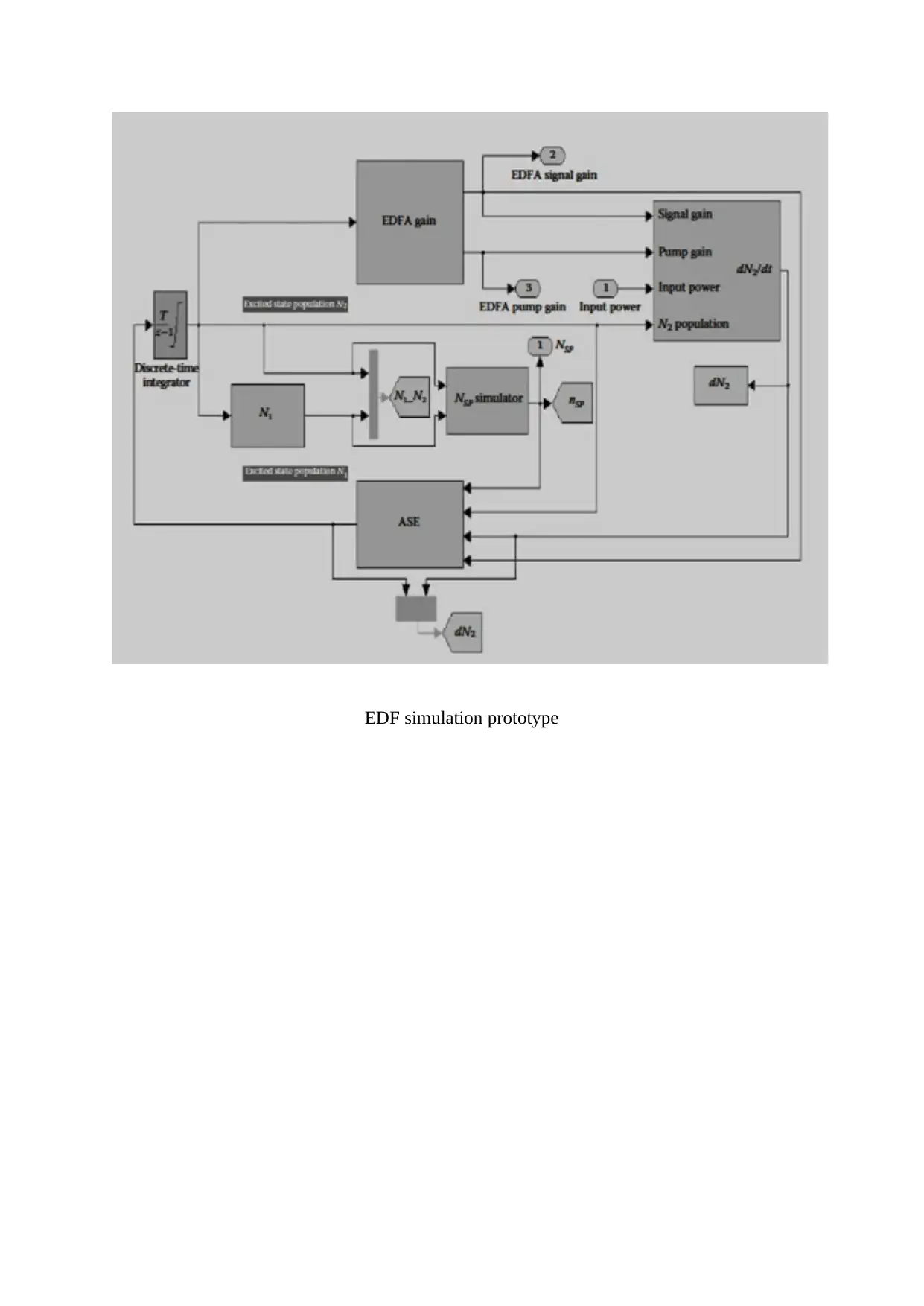
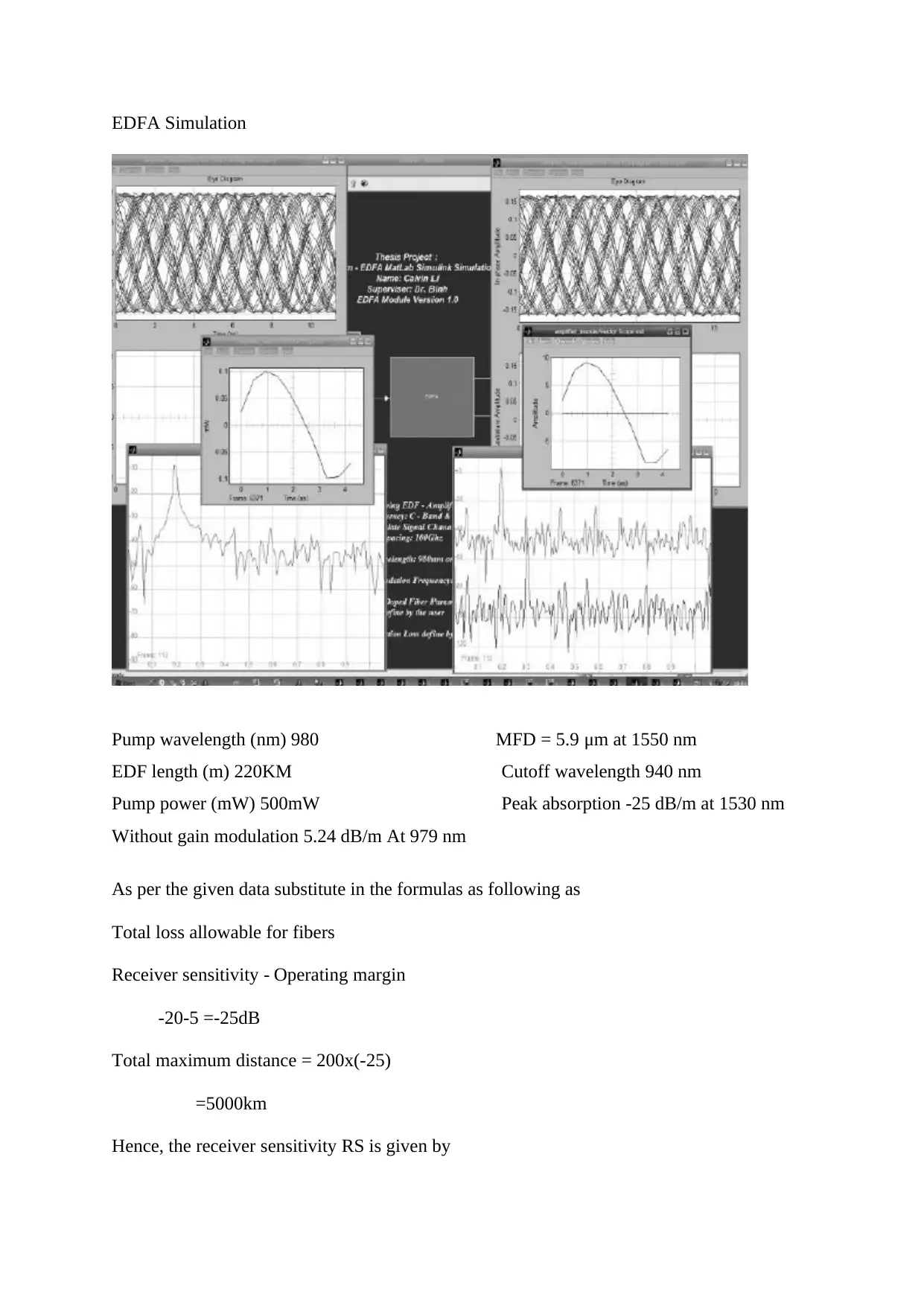
This report presents a detailed design and analysis of a Radio over Fiber (ROF) system for advanced optical communications. It covers key aspects such as optical source selection, power budget calculations, rise time/bandwidth budget, and Bit Error Rate (BER) and Signal to Noise Ratio (SNR) analysis using MATLAB simulations. The design incorporates essential fiber optic components like LED transmitters, PIN detectors, and step-index multimode fibers, considering factors such as transmission distance, optical wavelength, and loss budget. The report also explores EDFA simulation, dispersion budget, and the impact of various parameters on system performance, aiming for a reliable, upgradeable, and cost-effective design that meets customer needs and future expansion requirements. The document includes MATLAB codes for BER and SNR calculations, along with relevant graphs and figures to illustrate the system's performance.

Subject: Advanced Optical Communications Order id: 757091
1)
Introduction
Radio over fibre (ROF):
ROF is very attractive technique for wireless access network infrastructure, because
transmission of microwaves and millimetre-waves through optical fibres for a long distance is
very much simpler than the other existing techniques. ROF is a technique by which high
frequency signals are transmitted by means of optical components. A ROF system consists of
a Central Site (CS) and a Remote Site (RS)/ Base site (BS) user end connected by an optical
fiber link or network. The main optical components employed in RoF technology are the
laser transmitter, the Photo detectors and the optical fiber.
Basic Block Diagram of Radio over Fibre
Design criteria is depends upon two things
1) Data Rate
2) Link length
While at the time of a Design the following Parameters are required
Modulation format
System fidelity: BER, SNR
Cost
Upgradeability
Commercial availability
According task requirement design of a RoF as following as

As per given data
Bandwidth = 2 Gbits/sec
Length= 5000km
Selecting optical source:
LED at 850 nm is suitable for short distances. Its generates – 10 dBm optical power.
Selecting optical detector:
PIN-FER optical detector is reliable and has – 50 dBm sensitivity.
Selection optical fiber:
Step-index multimode fiber is selected. The fiber has bandwidth length product of
1000 (gb/s) km.
b)
Power Budget Calculations:
Link Power Budget:
The relation between the power margin between the optical transmitter output and the
minimum receiver sensitivity.
= Transmitter powerbin dBm
= Sensitivity of receiver in dBm for given BER
Maximum permissible loss
Power limited link length=

Rise Time/ Bandwidth Budget Calculation:
Rise-time budget:
The link power budget has been established, a system rise time analysis calculations are meet
the budget
=Detector
Above mentioned equation total rise time ‘tsys’ of the link is the root mean square of the rise
times from each contributor (ti ) to the pulse rise-time degradation
Bit Error Rate (BER):
Defined as the ratio of the number of errors in a given time interval (Ne) to the number of bits in that
time interval (Nt).
BER=
In general telecommunication applications the specified maximum BER falls in the range in
between .
For RZ data format
Bit rate R = B =1/ τ
Signal to Noise Ratio (SNR):
SNR is defined as the ratio of the average optical signal power to the average optical noise
power.
Here
I = Average Signal Power
= Optical Noise Power

Matlab code for BER, SNR
clear all
clc
r=randint(1,10000);
for i=1:10000
if r(i)==0
s(i)=-1;
else
s(i)=1;
end
end
k=1;
for snrdb=1:1:10;
v=1/(10^(snrdb/10));
x=awgn(s,snrdb,'measured');
y=x;
for j=1:10000
if y(j)>0
z(j)=1;
else
z(j)=0;
end
end
error=length(find(z~=r));
ber(k)=error/10000;
k=k+1;
end
snrdb=1:1:10;
snrlin=10.^(snrdb./10);
tber=0.5.*erfc(sqrt(snrlin));
semilogy(snrdb,ber,'-bo',snrdb,tber,'-mh')
grid on
title('task1');
xlabel('SNR');

ylabel('Bit error rate')
Matlab code for BER SNR Power graphs as following as
S=randint(1,20000);
mod=2*S-1;
snr=0:20;
Eb_No=10.^(snr/10);
for j=1:length(snr);
recvd=awgn(mod,snr(j),'measured');
No/2 variance)
for k=1:20000
if recvd(k)>0
demodulation(k)=1;
else
demodulation(k)=0;
end
end
[No_of_bits_corrupted(j) BER(j)]=biterr(S,demodulation);
q_x(j)=0.5*erfc(Eb_No(j)/sqrt(2));

end
figure
axis([0 20 0.0001 1]);
plot(snr,BER,'r');
title(‘power graph’)
xlabel('SNR')
ylabel('BER(log)');
semilogy(snr,BER,'r',snr,q_x,'g')

c)
While at the time design ROF Transmitter the following component are required
At the time design the system the following Fiber Optic components Requirements:
Transmission Distance
Optical Wavelength
Required Loss Budget
Optical Connectors
Fiber Type
Fiber Length
Installation Environment
Component Bandwidth Rise time
Transmitter 200MHxz 1.75 nsec
LED (850 nm) 100 MHz 3.50 nsec
Fiber cable 90 MHz 3.89 nsec
PIN detector 350 MHz 1.00 nsec
Receiver 180 MHz 1.94 nsec
Features of RZ codes in design in unipolar RZ data pattern a 1-bit is represented by a half-
period in either first or second half of the bit-period.
The below mentioned table will specify different distances sources and fiber link Capacity

The Gigabit Optical Communications required data collected from various manuals and some
text books are following as
1) Cisco Systems, Inc. Cisco Public Information
2) FISCHER FIBEROPTIC SERIES reference manuals
3) Optical Fiber Communications Principles and Practice Third edition John M. Senior
d)
The mentioned design as per our company requirement for upgrading existing one while at the
time of implementation of this project will consider all key points discussed in technical
review committee. Being a design engineer consider all the points of based on allocated budget
and future manpower and upgradability conditions. And also try meeting customer needs for
giving better services from our communication company.
Before implementation of this project discuss with my boss and other higher official in my
organization how it works the simple reliable upgradeable inexpensive design.

Subject: Advanced Optical Communications Order id: 757091
Assignment_2
a) As per the given data of the task as following as
An optical transmission system can be divided into three main subsystems
1) Optical transmitter,
2) Optical fiber channel,
3) Optical receiver,
In Optical transmitter the main function of an optical transmitter is to generate light waves
carrying a particular modulation format.
Simple block dia gram of optical transmission systems

An optical transmission system design
N1 simulation.
Recall the three state populations and the assumption that N3 is zero. The relation
between N1 and N2 is then N1 = Ntotal − N2
• Nsp simulation
According to the population inversion factor equation, N1 would equal N2. This would lead to
the result approaching infinity. Therefore, the [if statement] could limit the result to under 10.
Also, the population inversion factor would be greater than 10 in practice.

EDF simulation prototype

EDFA Simulation
Pump wavelength (nm) 980 MFD = 5.9 μm at 1550 nm
EDF length (m) 220KM Cutoff wavelength 940 nm
Pump power (mW) 500mW Peak absorption -25 dB/m at 1530 nm
Without gain modulation 5.24 dB/m At 979 nm
As per the given data substitute in the formulas as following as
Total loss allowable for fibers
Receiver sensitivity - Operating margin
-20-5 =-25dB
Total maximum distance = 200x(-25)
=5000km
Hence, the receiver sensitivity RS is given by

When =1Mw
Design description:
Notes: As the EDFA module can combine with other simulation blocks, the input data
stream can be replaced by any other device simulator block. To increase the execution
time, the run type in [normal mode], [accelerating mode], [from outside] in the option
menu can be changed.
Typical simulator screen shots of the Simulink EDFA simulator are given in Figures
The simulated results are based on practical EDFA parameters constructed in our laboratory
and some commercial amplifiers operating in the C-band. gives a set of the parameters
employed in the simulator, and the power generated at the output of the EDFA plotted versus
the input signal power with the wavelength of the input channel as a parameter is given in
Figures. The saturation is set at around −14 dBm as expected.
The EDFA gain obtained from the simulation agrees with that from the experiment, and the
only discrepancy is during low signal input power, this might be due to the internal setting of
the commercial device, which is unknown; all the other factors such as the absorption and
emission spectrum in the commercial EDFA may be slightly different from the simulator The
spectral gain is dependent on the stimulation emission factor. As the population inversion rate
changes with the signal wavelength, the gain peaks at 1528 nm Gain do not increase infinitely
with the increasing pump power as the ion density in erbium-doped fiber is constant. The
power pump just pushes the energy pumping ions to the higher energy state. Thus, if all the
ions have been pumped to the high state, then even

b)
The power budget obtained from the transmission link as following as

c)
Matlab code for BER, SNR
clear all

clc
r=randint(1,10000);
for i=1:10000
if r(i)==0
s(i)=-1;
else
s(i)=1;
end
end
k=1;
for snrdb=1:1:10;
v=1/(10^(snrdb/10));
x=awgn(s,snrdb,'measured');
y=x;
for j=1:10000
if y(j)>0
z(j)=1;
else
z(j)=0;
end
end
error=length(find(z~=r));
ber(k)=error/10000;
k=k+1;
end
snrdb=1:1:10;
snrlin=10.^(snrdb./10);
tber=0.5.*erfc(sqrt(snrlin));
semilogy(snrdb,ber,'-bo',snrdb,tber,'-mh')
grid on
title('task1');
xlabel('SNR');
ylabel('Bit error rate')

Matlab code for BER SNR Power graphs as following as
S=randint(1,20000);
mod=2*S-1;
snr=0:20;
Eb_No=10.^(snr/10);
for j=1:length(snr);
recvd=awgn(mod,snr(j),'measured');
No/2 variance)
for k=1:20000
if recvd(k)>0
demodulation(k)=1;
else
demodulation(k)=0;
end
end
[No_of_bits_corrupted(j) BER(j)]=biterr(S,demodulation);
q_x(j)=0.5*erfc(Eb_No(j)/sqrt(2));
end
figure

axis([0 20 0.0001 1]);
plot(snr,BER,'r');
title(‘power graph’)
xlabel('SNR')
ylabel('BER(log)');
semilogy(snr,BER,'r',snr,q_x,'g')
d)
Dispersion Budget: dispersion budget for different optical transmission structures.

The relationship between the dispersion, the bit rate, and the bandwidth. For on–off keying
(OOK), the bandwidth Δf of the detection system can be about 1/2 the bit rate (pulse
repetition rate). The relationship of B,L ≤1/4|DT|σλ can be used, or the bit rate BR can be
approximately written as
=
Reference text book
Optical Fiber Communication Systems with MATLAB® and Simulink® Models
2nd Edition Le Nguyen Binh
Optical Wireless Communications System and Channel Modelling with MATLAB®
Z. Ghassemlooy W. Popoola S. Rajbhandari