Individual Exercise 1: Time Series Analysis of Digester 5 Level Data

This report presents a comprehensive analysis of the D2Dig5:PTPV (Digester 5 level) data from the QAL digestion area (#2), focusing on time series analysis techniques. The analysis includes visual observation of the data's dynamics, spectral analysis to identify frequency components, and an examination of potential effects of filtering high-frequency noise. The report also addresses the presence of gross errors and outliers within the dataset. The study explores the stationarity of the time series and employs methods such as Moving Averages (MA), Autoregressive (AR), and Autoregressive Moving Averages (ARMA) models, along with the Box-Jenkins ARIMA process to understand the data's characteristics and model its behavior. The report also discusses concepts such as lag, differencing, trend, seasonality, and cyclical and irregular variations. The goal is to provide insights into the time series character, potential origins of the dynamics, and identify the best ARIMA model for forecasting. The analysis is performed in Rstudio, and the report includes detailed commentary and insights regarding the time series characteristics.

Running head: PROCESS MODELLING AND SIMULATION 1
Process Modeling and Simulation
Student:
Professor:
Institution Affiliation:
Course:
Date:

PROCESS MODELLING AND SIMULATION 2
Process Modeling and Simulation
Theoretical Framework
This part of the paper critically examines time series basics which are comprised of the
assumptions, principles as well as conditions necessary for the analysis, and also the processes
coupled in the use of MA, ARIMA and also ARMA or even AR. The set of variables applied in
this study analysis are D2Dig5: PTPV (Digester 5 level) on the QAL digestion area (#2) data set
to understand its characteristics and provide insights from those analyses.
Sources as well as Nature the used dataset
The data in this analysis was secondary obtained information of a flash tank of a given
plant. The variable hourly, digester flow cut, low-pressure heater swap, and high-pressure FT
online; each of which was distinct from one another. The named variables were analyzed
separately. The number of observations on hourly data was 2990; digester flow cut 10096, high-
pressure FT online 7295, and low-pressure heater swap 10096 records.
Basic Definitions and Analysis Concepts
Time Series
This analysis involves approaches for breaking down a data chain into mechanisms with
easily understandable lots allowing recognition of movements, and hence setting forecasts and
also approximations of a given study. The key significance of time series assessment is the
explanation of statistics plots underlying framework with the help of estimation of prospect
values on the basis of previously known data. This is possible through the application of time
series models namely; MA, GARCH, AR, CGARCH, ARIMA, TARCH, FIGARCH as well as
EGARCH (Shumway & Stoffer, 2017). This analysis is based on models MA, ARMA and AR.
Lag

PROCESS MODELLING AND SIMULATION 3
This is the time phases amid two data points. For example, lag 1 could be between Xt
and Xt-1 while lag 2 is between Xt and Xt-2. It is as well possible to lag or else to forward time
series i.e. Xt as well as Xt+1. For this study, the data point, Xt, is dependent on preceding point
observation, Yt-1.
Differencing
In simple terms, this means subtracting the previous observation value from future
observation. Generally, it involves the computation of alterations of pairs of the various
observation pairs within a certain lag in order to obtain non-stationary and stationary series
(Mills, 2015).
Stationary and Non-stationary Series
Stationary chain diverges on the subject of an unremitting normal point, neither
dwindling nor increasing steadily through time, with a lasting variance. On the other hand, non-
stationary series, have methodical trends, such as linear, and quadratic (Mills, 2015). Non-
stationary series that can possibly be made stationary through performing a differencing and
referring to the new data as non-stationary in a similar sense (Mills, 2015). A non-stationary
approach with a deterministic movement tends to stationary after eliminating the drift. The
following describes an example of these transformations.
Xt = α + βt + εt is changed into a stationary approach by deducting the movement (trend).
Βt, Xt - βt = α +εt.
No point is gone astray when the transformation (detrending) is applied to change time-series
data from non-stationary to stationary. Non-stationary statistics, as a general rule in statistics, are
impulsive and cannot be predicted or modeled (Mills, 2015).
The Trend (d)

PROCESS MODELLING AND SIMULATION 4
The trend is simply the fundamental long-term move or series. The QAL digestion area
(#2) described the trend as a non-current tendency in a time series short of schedule associated
and uneven impacts and is a likeness of the fundamental point (Hunter, Burke & Canepa, 2017).
It is the outcome of effects such as populace progression, price rise, and overall financial
variations. A model with two trend terms has to be differenced two times to make it stationary.
The first difference eliminates a linear trend; the second difference removes the quadratic trend,
and so on.
Seasonality Variation (S)
A seasonal effect is an orderly and calendar associated effect. An example of seasonal
variation includes the sharp growth in most retail series that happens around December in
reaction to the Christmas season (Cohen, 2014). The seasonal modification can be stated as the
procedure of approximating and then eliminating from a forecasting model the influences that
are orderly and calendar associated. Recorded statistics requires being seasonally modified as
seasonal impacts can hide both the true fundamental trends in the model, and definite non-
seasonal features that may be of attention to statistical forecasters (Palma, 2016). Seasonality in a
forecasting model can be acknowledged by frequently spread out heights and troughs which have
a reliable pattern (Cohen, 2014). Other procedures which can be applied in time series
examination to sense seasonality include:
i. A seasonal models design is a focused method for viewing seasonality.
ii. Multiple box plots can be applied as a substitute for the seasonal approaches plot to sense
seasonality.
iii. Seasonality is also detected by the help of the autocorrelation plot.
Cyclical Variations (C)

PROCESS MODELLING AND SIMULATION 5
Cyclical variations are the short term deviations (rises and falls) which occur in the data
that is not at a fixed time. They usually occur as a result of unforeseen or unpredictable activities
such as those linked with the business cycle sharp increase in inflation and stock price (Cohen,
2014). The main alteration between the seasonal and cyclical variation is the fact that the former
is of a continuous length and recurs at regular intervals, while the latter differs in measurement
(Palma, 2016). More so, the length of a cycle is averagely longer than that of seasonality with the
magnitude of a cycle typically being more variable than that of seasonal difference.
Irregular Variations (I)
The irregular constituent also referred to as the residual is remainders later when the
seasonal and tendency components of a time series have been projected and detached. It comes
from current variations in the models that are neither orderly nor foreseeable (Palma, 2016). In
an extremely irregular model, the oscillations mentioned can control trends that will cover the
seasonality and movement.
Common Assumptions in Time Series Techniques
A collective assumption in most forecasting modeling practices is that the statistics used
are stationary. A stationary progression has the characteristics that the autocorrelation mean, and
variance designs which do not vary with time (Palma, 2016). Then, stationarity can be then
described in statistical form as follows.
A particular variable is stationary is have the following properties.
i. The mean μt=E( Xt ¿
ii. The variance δ t=var ( Xt )=γ (0)
iii. The autocovariance, cover ( Xt 1 , Xt 2 )= γ (t1 , t2)
Autocorrelation Function (ACF)

PROCESS MODELLING AND SIMULATION 6
Autocorrelation can be described as the association of a forecasting model with its
historical and prospect data points. Autocorrelation is at times described in the as serial
association or lagged correlation which denotes the connection between members of a series of
numbers sorted about time (Palma, 2016). The design of autocorrelations in a forecasting model
at many pauses; the association at lag 1, then the correlation at lag 2 in that order (Cohen, 2014,
p. 18). Associations among consecutive scores at diverse intervals. Lag 1 autocorrelation
constant is comparable to the association between the duos of scores at contiguous levels at a
particular period;
γ Xt , Xt −1 Where t=1, 2, 3…
The study will apply the following tools in evaluating autocorrelation of the time series data.
i. The time series plot,
ii. The lagged scatter plot, and
iii. 3.The autocorrelation function
The correlation between Xt and Xt + k is computed by,
γk=
∑
t=1
N−K
( Xt −¯x)( X t+ k−¯x)
∑
t=1
N
( Xt−¯x )2
Where ¯x is the mean of the first N – 1 data points. The correlation constant described above
measure association between consecutive statistics it is referred to as the autocorrelation constant
or sequential correspondence factor.
Precisely, partial autocorrelations are suitable in classifying the pattern of an autoregressive
series. The incomplete autocorrelation of autoregressive (p) progression is nil at lag p+1 or more
(Cohen, 2014).

PROCESS MODELLING AND SIMULATION 7
Time Series Models
The following approaches will be applied in displaying the variables of the QAL digestion area
(#2) var time series data. The best ARIMA model was to be used in forecasting future climate
change variables.
Moving Averages (MA) Models
This method is composed of a theoretical lined reversion of a particular current
observation of MA white noise which can as well be referred to as haphazard tremors of earlier
figures of a dataset. In line with that, the random shocks observed in extreme points are assumed
to come of a related distribution, typically a normal scattering with an invariable scale as well as
a nil point (Cohen, 2014). The distinguishing factor of the method is random shocks are stretched
to the prospect values of forecast model(s). Plots of the MA approximations are more complex as
compared to the AR series since the error points are unnoticeable (Cohen, 2014). Therefore, it is
an implication that the unlined iterative design events should be used instead of the linear least
squares. MA series, as well have lesser comprehensible explanations as compared to
autoregressive designs. For those reasons, MA is a standard approach of coming up with a time
series dataset containing only a single variable.
The general formula is given below:
Xt =β0−Et −β1 Et −1−β2 Et−2−…−βq Et−q
Whereby;
Xt : time series,
Et −i: white noise also referred to as disturbances,
βi ' s: model parameters.
Random variables Ei ' s usually scaled such that β0=1

PROCESS MODELLING AND SIMULATION 8
Autoregressive (AR) Models
This is just a lined reversion a given present observation of the form Xt in relation to one
previously analyzed data points or more of the series in the model (Xt-i). The observation p is
said to be AR series direction (Hunter, Burke & Canepa, 2017). Autoregressive methodologies
could be assessed in the application of any of the discussed methods, count standard lined least-
squares processes. Further, these approaches have got a frank elucidation. A collective technique
for scheming a time series comprising of a univariate, AR series. The general formula is defined
as below;
Xt =α0 +α1 Xt + α2 Xt −1+α3 Xt −3+…+αP Xt −P +Et
Whereby
Xt : time series,
α i' s: Model parameters,
Et : white noise.
Autoregressive Moving Averages Models- ARMA
Autoregressive as well as Moving Average (ARMA) measures can be combined to result in
useful univariate class methods (proposed by Box and Jenkins), referred to as ARMA events
(Hunter, Burke & Canepa, 2017).
The time series Xt which is a representation of ARMA (p, q) modeling is estimated in the format
below.
Xt =δ+α 1 X t +α 2 X t−1 +α 3 X t−3 +…+αP X t−P + Et + β0 Et + β1 Et−1 +β2 Et−2 +…+ βq Et −q
The other model which was applied in the modeling of the QAL digestion area (#2) dataset
variables is the ARIMA.
Box-Jenkins ARIMA Process

PROCESS MODELLING AND SIMULATION 9
In statistical econometrics, normally, the ARIMA model is a summary of this time series
analysis of any given study. These systems are applied in given situations in which statistics
inhibit proof of non-stationarity, having the initial design phase is functional in the elimination of
non-stationarity.
Box-Jenkins Modeling Approach
The Box-Jenkins model applies iterative three-stage displaying approach which is described
below.
i. Model forming and choice- ensuring the factors are fixed, recognizing seasonality in the
response models (seasonally transformation A if it crucial), and by designs of the auto-
correlation and restricted auto-correlation purposes of the response models to determine
which one if any AR or MA constituent would be applied in the approach (Hunter, Burke
& Canepa, 2017).
ii. Factor approximation via calculating procedures to reach constants which best
approximates the chosen ARIMA approach
iii. Approach evaluation by assessing if the projected model follows the stipulations of a
fixed method involving only one variable.
Box-Jenkins approach Documentation
Stationarity and Seasonality
The initial phase is modeling a Box–Jenkins approach is to find out when the forecasting model
is fixed as well as determining if there is any important seasonality which requires being
displayed.
Identifying Stationarity

PROCESS MODELLING AND SIMULATION 10
In time series, stationarity can be evaluated from a course structure graph. The course
system design is supposed to indicate a continuous position and measure. Also, it would be
sensed from an auto-correlation graph. Precisely, non-stationarity is frequently designated by an
auto-correlation scheme with a relaxed decline (Gooijer, 2017). The KPSS evaluation for the H0
of a stationary series versus a substitute of fundamental cause composed of the Philips-Peron
evaluation for the H0 of a component root beside the alternate of a still sequence (Gooijer, 2017).
The basis for making the decision for the KPSS examination is that if the value of p of its
evaluation measurement is more than the acute observation, for instance a p-value of 0.05 then
cast-off the H0 of taking a smooth stationary sequence and settle that the H1 that it has an origin
of 1 (Gooijer, 2017). The Philips-Peron evaluation, on the other side, assesses the H0 of
elemental root versus an H1 of stationarity by declining the H0 if its value of p is smaller than the
acute observation selected.
Seasonal Differencing
During the approach documentation phase, the objective is to sense seasonality, when it
is present, and to recognize the direction for the periodic AR and cyclical MA factors. An
example is, for monthly statistics one normally comprises a cyclic autoregressive 12 point or on
the other hand a seasonal MA 12 term (Hunter, Burke & Canepa, 2017).
Recognizing p and q
When seasonality, as well as stationarity assessed, is over, the subsequent level is to recognize
the direction that is the p and q of the AR plus MA components (Hunter, Burke & Canepa,
2017). These are evaluated by assessing the observations of the autocorrelations and the semi-
associations with their consistent graphs as described below.
Auto-correlation and Incomplete Auto-correlation Graphs

PROCESS MODELLING AND SIMULATION 11
Main ways for performing this analysis are the auto-correlation graph as well as the
fractional auto-correlation graph. The trial auto-correlation graph plus the trial incomplete auto-
correlation design are associated with the hypothetical performance of these graphs if the
direction is determined (Hunter, Burke & Canepa, 2017). The time series analysis was performed
using rstudio.
Time Series Analysis of D2Dig5: PTPV (Digester 5 level)
D2Dig5: PTPV (Digester 5 level) is found on hourly data, low-pressure heater swap, and high
pressure online from the entire dataset. The time series analysis for D2Dig5: PTPV (Digester 5
level) in each of these data sets is described below;
Hourly Data

PROCESS MODELLING AND SIMULATION 12
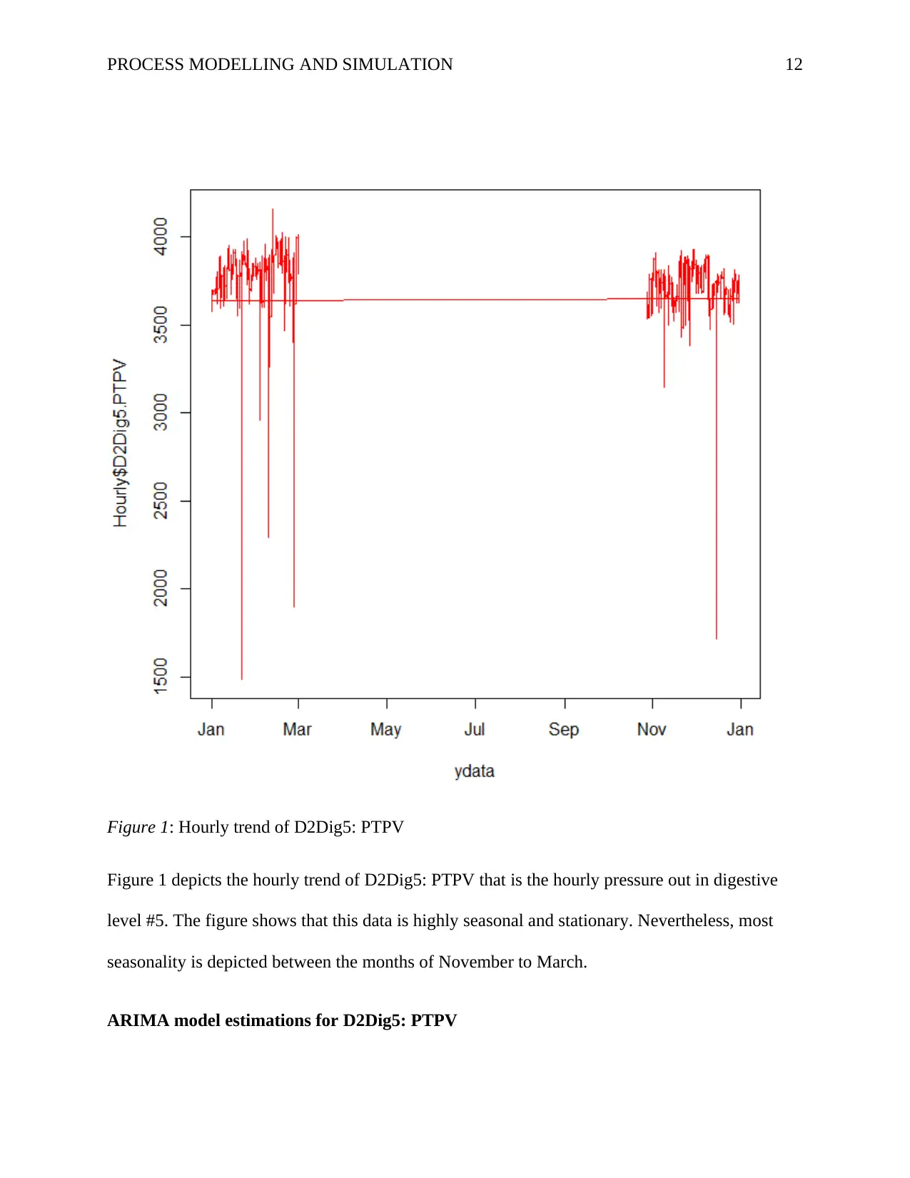
Figure 1: Hourly trend of D2Dig5: PTPV
Figure 1 depicts the hourly trend of D2Dig5: PTPV that is the hourly pressure out in digestive
level #5. The figure shows that this data is highly seasonal and stationary. Nevertheless, most
seasonality is depicted between the months of November to March.
ARIMA model estimations for D2Dig5: PTPV