2019 Advanced Robotics Project: Neural Networks for Robot Control
VerifiedAdded on 2022/11/16
|17
|2553
|290
Project
AI Summary
This project report details the implementation of neural networks for controlling a two-link robot. The study begins with the development of a SIMULINK model based on the robot's dynamic equations, followed by the implementation of a computed-torque controller (CTC). The core of the project involves designing and implementing a neural network controller (NNC) to perform CTC, which is then integrated into the SIMULINK model. The report covers the robot's kinematic and dynamic equations, the CTC design, and the neural network controller's architecture, training, and implementation using a backpropagation algorithm. The MATLAB simulations for the two-link arm robot based on the kinematic dynamic equations of the system are illustrated. The results demonstrate the effectiveness of the NNC in controlling the robot's movements, addressing uncertainties, and achieving desired performance. The project also highlights the advantages of neural network controllers in achieving precise, accurate, and robust control, including the ability to handle disturbances and model parameter variations.
NEURAL NETWORKS
FOR ROBOT CONTROL
[Year]
FOR ROBOT CONTROL
[Year]
Paraphrase This Document
Need a fresh take? Get an instant paraphrase of this document with our AI Paraphraser
INTRODUCTION
The Robot institute of America describes the two link robot as a multifunctional manipulator that
can be programmed and reprogrammed with the aim of carrying out repetitive human tasks
especially in the industrial settings. The programmable instructions are embedded in the
mechanical structure with limited memory. Such robots are implemented in dangerous areas for
space exploration, disarming of bombs, disaster or debris cleanup, and chemical spill cleanup.
Further, they are used in carrying out repetitive industrial or human residential tasks and tasks
that require high precision or extremely high speeds and consistency. The performance of a robot
is measured based on the working volume, the speed and acceleration, accuracy, repeatability,
and the resolution.
The initial designs of the robot enabled instructions to be given to the machines in form of
numeric codes. The system was an open-loop system whose results were not measured against
the intended output. There are different types of robots namely the industrial, locomotion or
exploration, medical, and entertainment. An open loop system may not perform well or as
intended hence the need for robotic control. The robotic control ensures path planning and
navigation for the mobile robots, compensation for the robot’s dynamic properties, trajectory
monitoring to avoid obstacles externally, and to have a direct control of the forces or the
displacements of the manipulator.
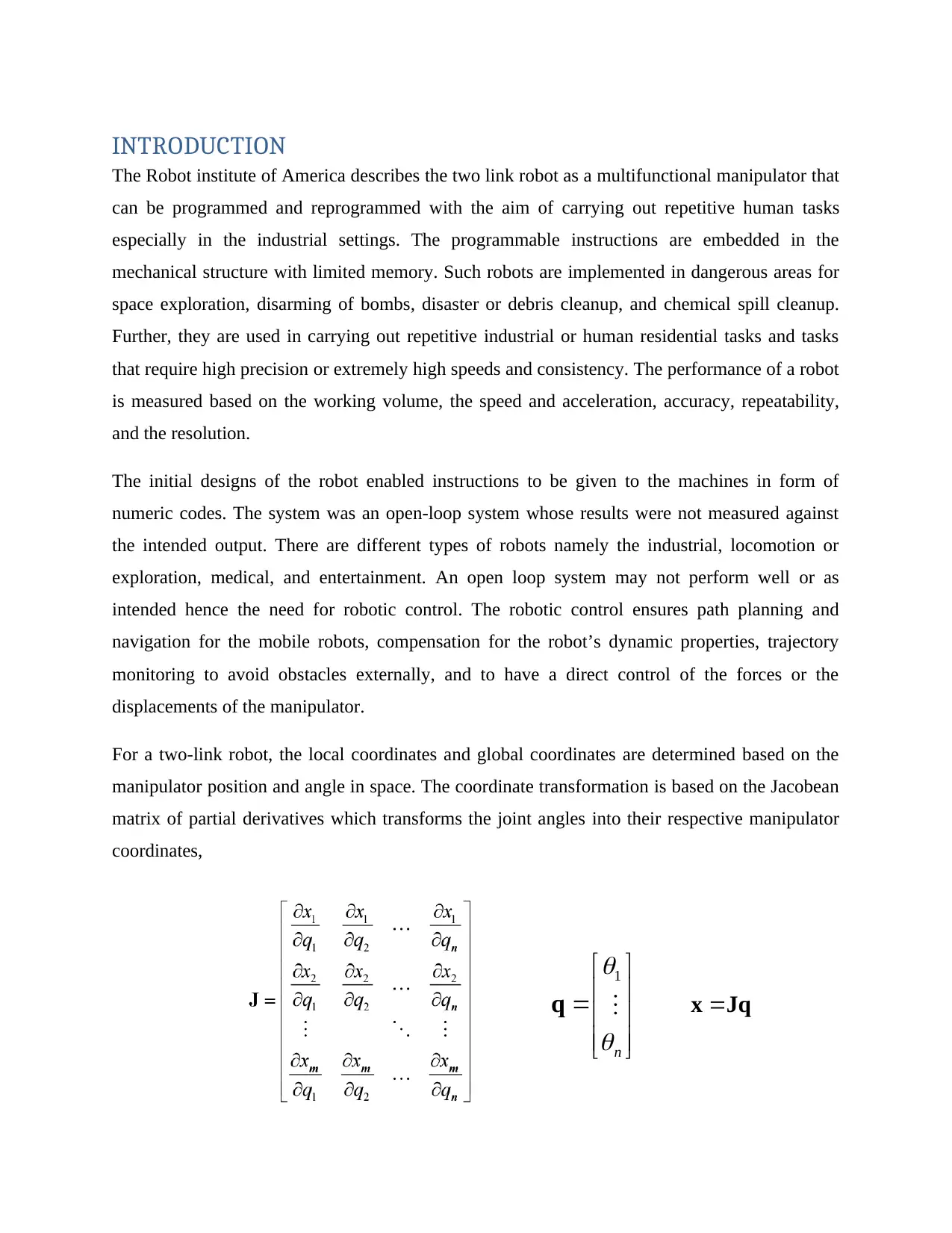
For a two-link robot, the local coordinates and global coordinates are determined based on the
manipulator position and angle in space. The coordinate transformation is based on the Jacobean
matrix of partial derivatives which transforms the joint angles into their respective manipulator
coordinates,
Jqx
n
1
q
The Robot institute of America describes the two link robot as a multifunctional manipulator that
can be programmed and reprogrammed with the aim of carrying out repetitive human tasks
especially in the industrial settings. The programmable instructions are embedded in the
mechanical structure with limited memory. Such robots are implemented in dangerous areas for
space exploration, disarming of bombs, disaster or debris cleanup, and chemical spill cleanup.
Further, they are used in carrying out repetitive industrial or human residential tasks and tasks
that require high precision or extremely high speeds and consistency. The performance of a robot
is measured based on the working volume, the speed and acceleration, accuracy, repeatability,
and the resolution.
The initial designs of the robot enabled instructions to be given to the machines in form of
numeric codes. The system was an open-loop system whose results were not measured against
the intended output. There are different types of robots namely the industrial, locomotion or
exploration, medical, and entertainment. An open loop system may not perform well or as
intended hence the need for robotic control. The robotic control ensures path planning and
navigation for the mobile robots, compensation for the robot’s dynamic properties, trajectory
monitoring to avoid obstacles externally, and to have a direct control of the forces or the
displacements of the manipulator.
For a two-link robot, the local coordinates and global coordinates are determined based on the
manipulator position and angle in space. The coordinate transformation is based on the Jacobean
matrix of partial derivatives which transforms the joint angles into their respective manipulator
coordinates,
Jqx
n
1
q
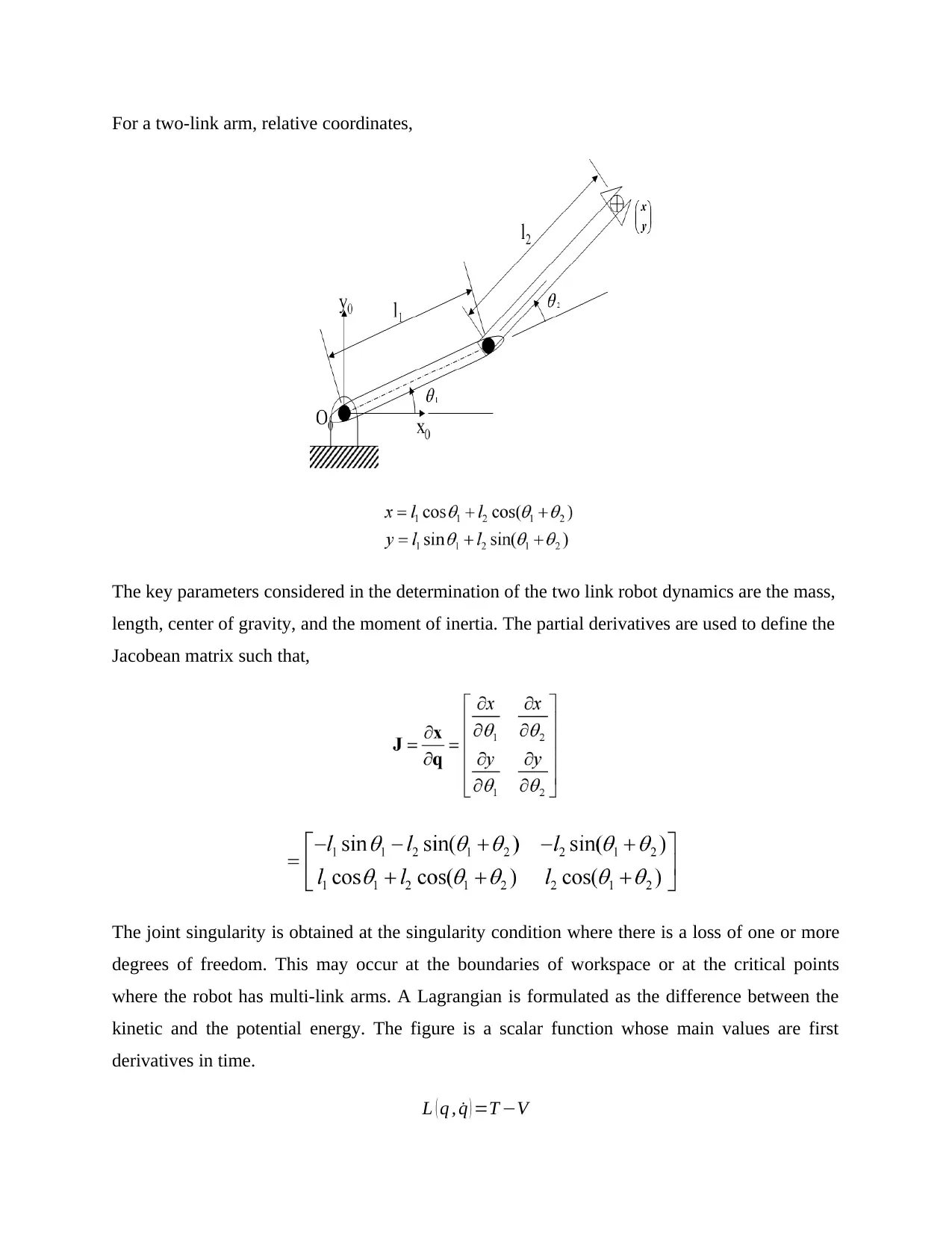
For a two-link arm, relative coordinates,
The key parameters considered in the determination of the two link robot dynamics are the mass,
length, center of gravity, and the moment of inertia. The partial derivatives are used to define the
Jacobean matrix such that,
The joint singularity is obtained at the singularity condition where there is a loss of one or more
degrees of freedom. This may occur at the boundaries of workspace or at the critical points
where the robot has multi-link arms. A Lagrangian is formulated as the difference between the
kinetic and the potential energy. The figure is a scalar function whose main values are first
derivatives in time.
L ( q , ˙q ) =T −V
⊘ This is a preview!⊘
Do you want full access?
Subscribe today to unlock all pages.
Trusted by 1+ million students worldwide
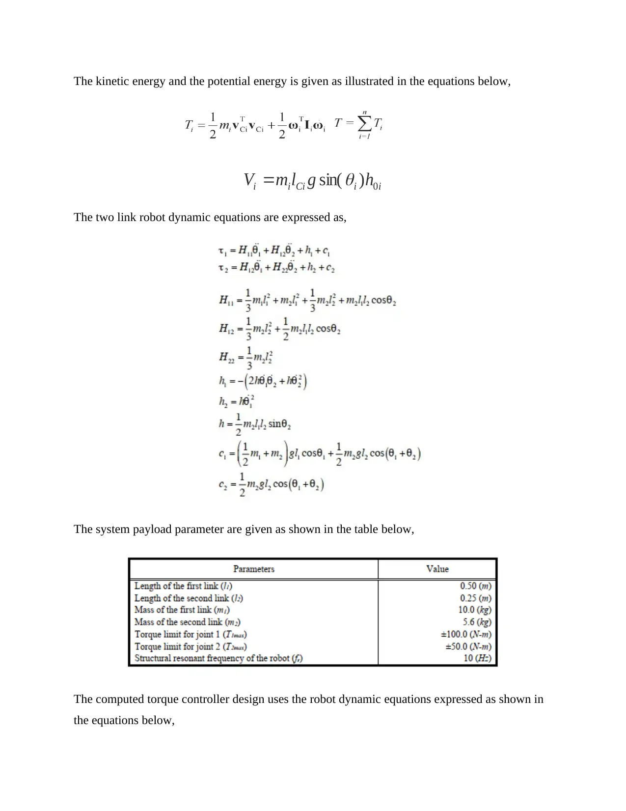
The kinetic energy and the potential energy is given as illustrated in the equations below,
iiCiii hglmV 0)sin(
The two link robot dynamic equations are expressed as,
The system payload parameter are given as shown in the table below,
The computed torque controller design uses the robot dynamic equations expressed as shown in
the equations below,
iiCiii hglmV 0)sin(
The two link robot dynamic equations are expressed as,
The system payload parameter are given as shown in the table below,
The computed torque controller design uses the robot dynamic equations expressed as shown in
the equations below,
Paraphrase This Document
Need a fresh take? Get an instant paraphrase of this document with our AI Paraphraser
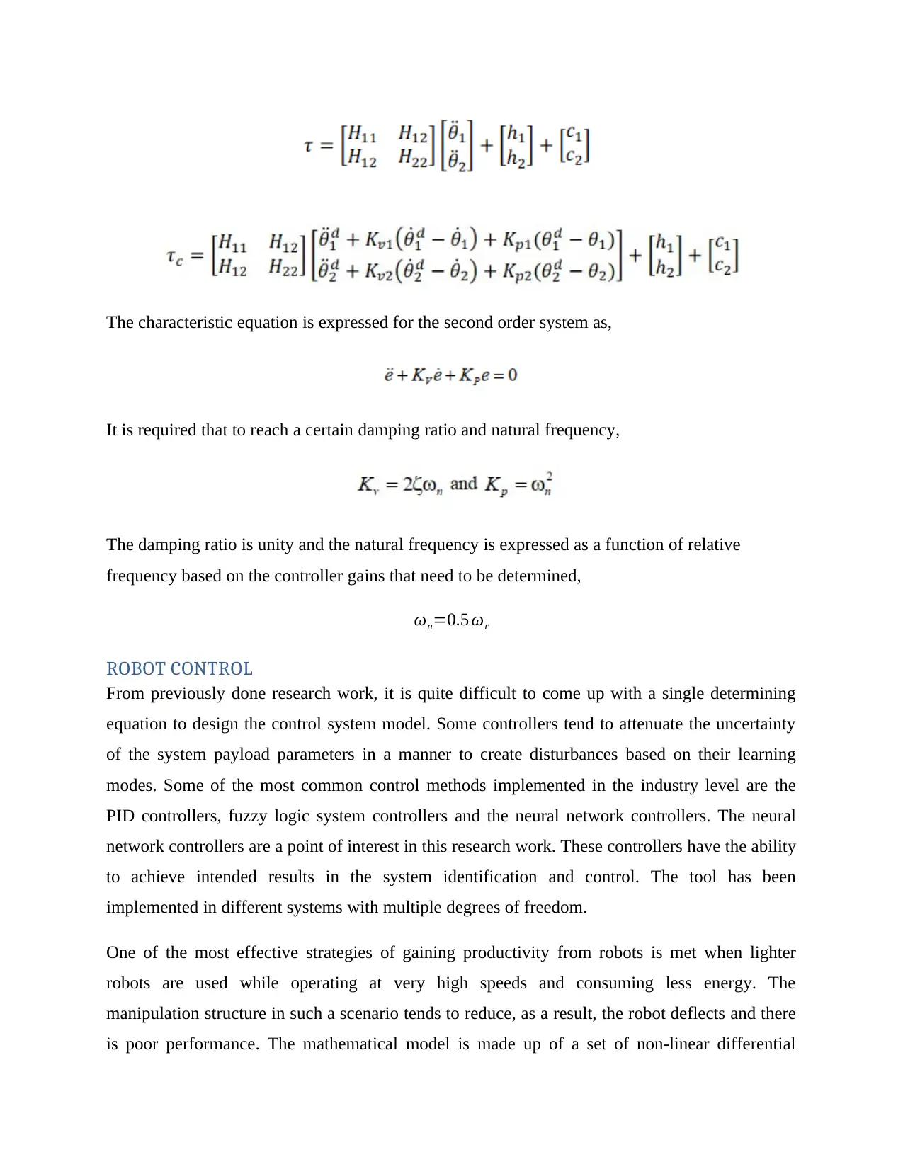
The characteristic equation is expressed for the second order system as,
It is required that to reach a certain damping ratio and natural frequency,
The damping ratio is unity and the natural frequency is expressed as a function of relative
frequency based on the controller gains that need to be determined,
ωn=0.5 ωr
ROBOT CONTROL
From previously done research work, it is quite difficult to come up with a single determining
equation to design the control system model. Some controllers tend to attenuate the uncertainty
of the system payload parameters in a manner to create disturbances based on their learning
modes. Some of the most common control methods implemented in the industry level are the
PID controllers, fuzzy logic system controllers and the neural network controllers. The neural
network controllers are a point of interest in this research work. These controllers have the ability
to achieve intended results in the system identification and control. The tool has been
implemented in different systems with multiple degrees of freedom.
One of the most effective strategies of gaining productivity from robots is met when lighter
robots are used while operating at very high speeds and consuming less energy. The
manipulation structure in such a scenario tends to reduce, as a result, the robot deflects and there
is poor performance. The mathematical model is made up of a set of non-linear differential
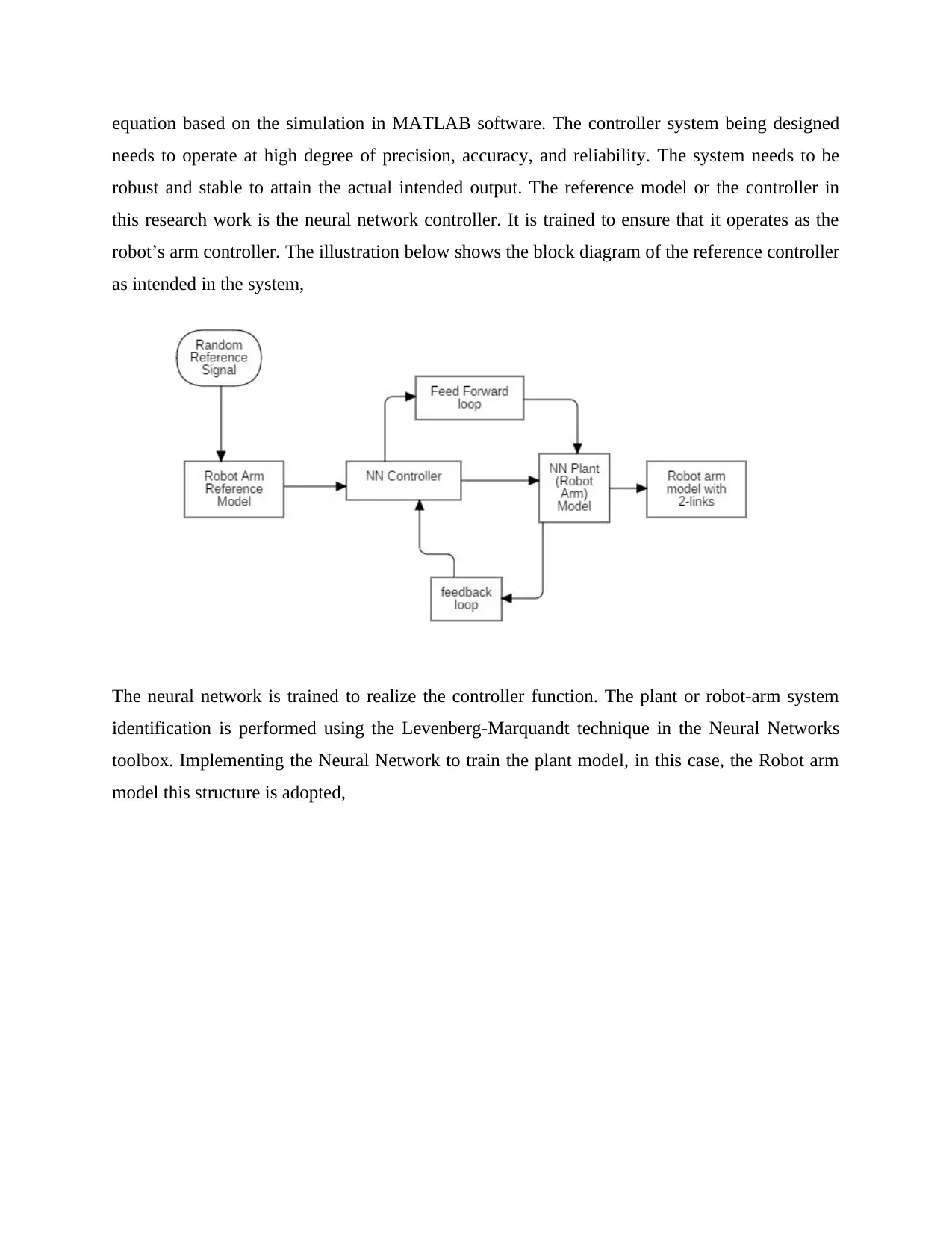
equation based on the simulation in MATLAB software. The controller system being designed
needs to operate at high degree of precision, accuracy, and reliability. The system needs to be
robust and stable to attain the actual intended output. The reference model or the controller in
this research work is the neural network controller. It is trained to ensure that it operates as the
robot’s arm controller. The illustration below shows the block diagram of the reference controller
as intended in the system,
The neural network is trained to realize the controller function. The plant or robot-arm system
identification is performed using the Levenberg-Marquandt technique in the Neural Networks
toolbox. Implementing the Neural Network to train the plant model, in this case, the Robot arm
model this structure is adopted,
⊘ This is a preview!⊘
Do you want full access?
Subscribe today to unlock all pages.
Trusted by 1+ million students worldwide
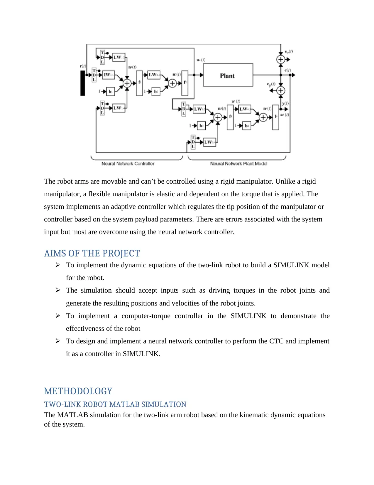
The robot arms are movable and can’t be controlled using a rigid manipulator. Unlike a rigid
manipulator, a flexible manipulator is elastic and dependent on the torque that is applied. The
system implements an adaptive controller which regulates the tip position of the manipulator or
controller based on the system payload parameters. There are errors associated with the system
input but most are overcome using the neural network controller.
AIMS OF THE PROJECT
To implement the dynamic equations of the two-link robot to build a SIMULINK model
for the robot.
The simulation should accept inputs such as driving torques in the robot joints and
generate the resulting positions and velocities of the robot joints.
To implement a computer-torque controller in the SIMULINK to demonstrate the
effectiveness of the robot
To design and implement a neural network controller to perform the CTC and implement
it as a controller in SIMULINK.
METHODOLOGY
TWO-LINK ROBOT MATLAB SIMULATION
The MATLAB simulation for the two-link arm robot based on the kinematic dynamic equations
of the system.
Paraphrase This Document
Need a fresh take? Get an instant paraphrase of this document with our AI Paraphraser
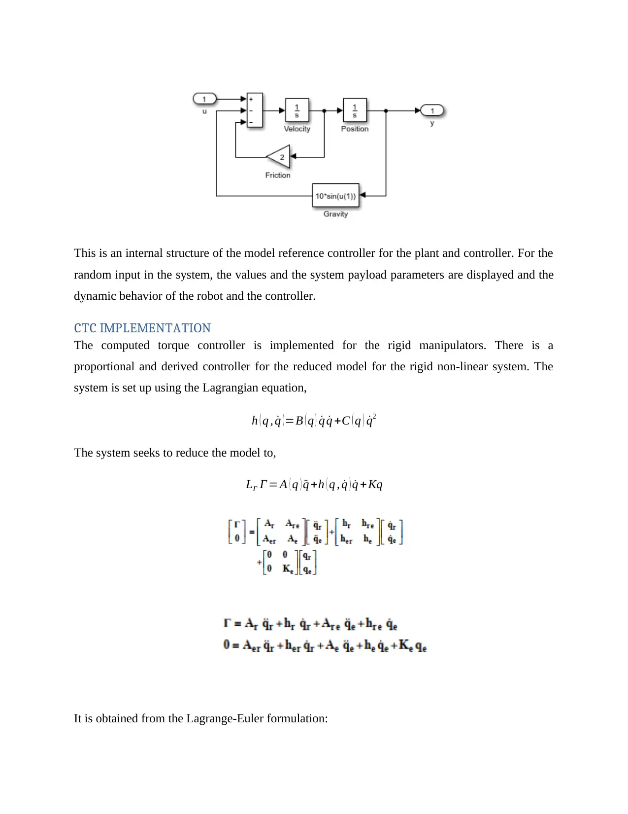
This is an internal structure of the model reference controller for the plant and controller. For the
random input in the system, the values and the system payload parameters are displayed and the
dynamic behavior of the robot and the controller.
CTC IMPLEMENTATION
The computed torque controller is implemented for the rigid manipulators. There is a
proportional and derived controller for the reduced model for the rigid non-linear system. The
system is set up using the Lagrangian equation,
h ( q , ˙q )=B ( q ) ˙q ˙q +C ( q ) ˙q2
The system seeks to reduce the model to,
LΓ Γ = A ( q ) ¨q +h ( q , ˙q ) ˙q + Kq
It is obtained from the Lagrange-Euler formulation:
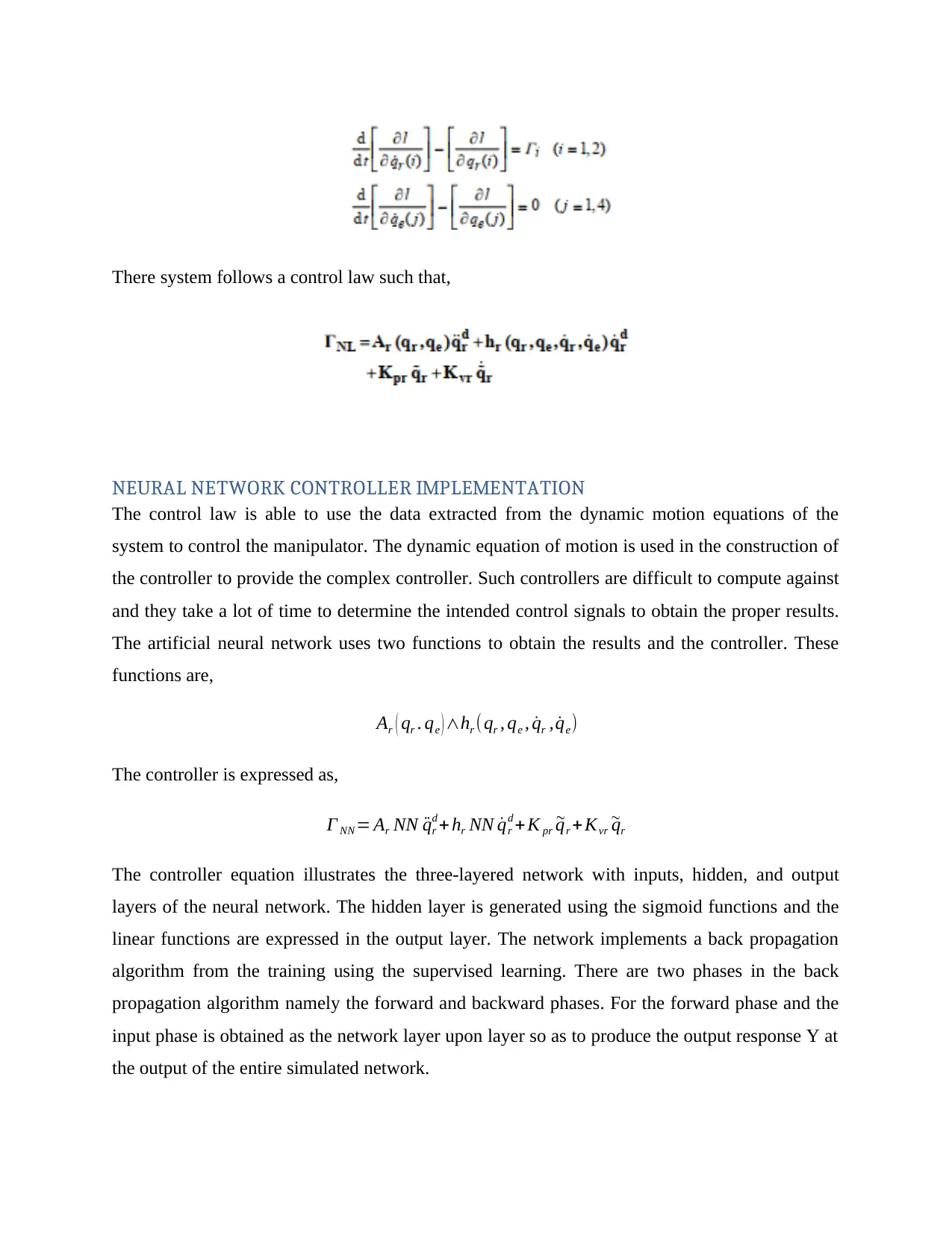
There system follows a control law such that,
NEURAL NETWORK CONTROLLER IMPLEMENTATION
The control law is able to use the data extracted from the dynamic motion equations of the
system to control the manipulator. The dynamic equation of motion is used in the construction of
the controller to provide the complex controller. Such controllers are difficult to compute against
and they take a lot of time to determine the intended control signals to obtain the proper results.
The artificial neural network uses two functions to obtain the results and the controller. These
functions are,
Ar ( qr . qe ) ∧hr (qr , qe , ˙qr , ˙qe)
The controller is expressed as,
Γ NN = Ar NN ¨qr
d + hr NN ˙qr
d + K pr ~qr +Kvr ~qr
The controller equation illustrates the three-layered network with inputs, hidden, and output
layers of the neural network. The hidden layer is generated using the sigmoid functions and the
linear functions are expressed in the output layer. The network implements a back propagation
algorithm from the training using the supervised learning. There are two phases in the back
propagation algorithm namely the forward and backward phases. For the forward phase and the
input phase is obtained as the network layer upon layer so as to produce the output response Y at
the output of the entire simulated network.
⊘ This is a preview!⊘
Do you want full access?
Subscribe today to unlock all pages.
Trusted by 1+ million students worldwide
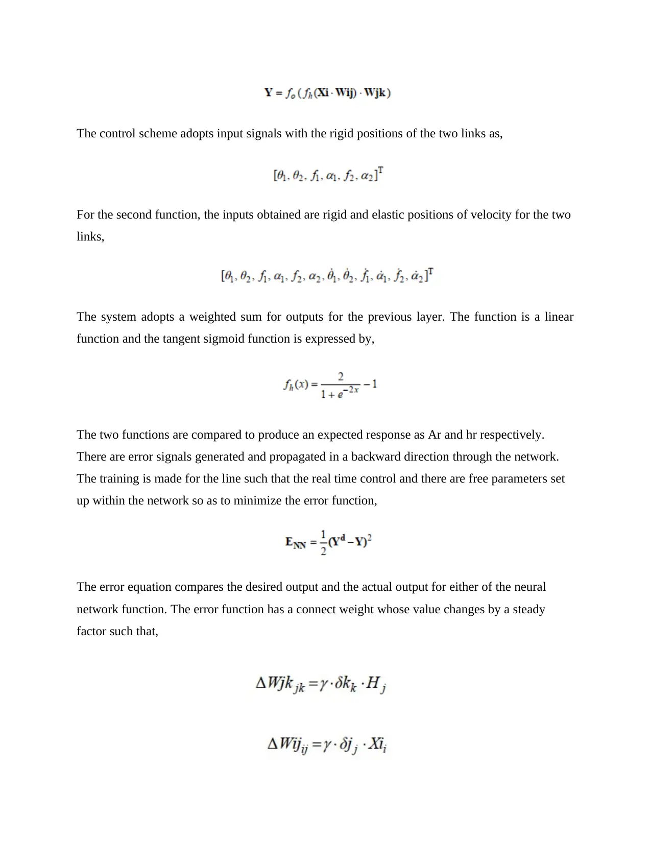
The control scheme adopts input signals with the rigid positions of the two links as,
For the second function, the inputs obtained are rigid and elastic positions of velocity for the two
links,
The system adopts a weighted sum for outputs for the previous layer. The function is a linear
function and the tangent sigmoid function is expressed by,
The two functions are compared to produce an expected response as Ar and hr respectively.
There are error signals generated and propagated in a backward direction through the network.
The training is made for the line such that the real time control and there are free parameters set
up within the network so as to minimize the error function,
The error equation compares the desired output and the actual output for either of the neural
network function. The error function has a connect weight whose value changes by a steady
factor such that,
Paraphrase This Document
Need a fresh take? Get an instant paraphrase of this document with our AI Paraphraser
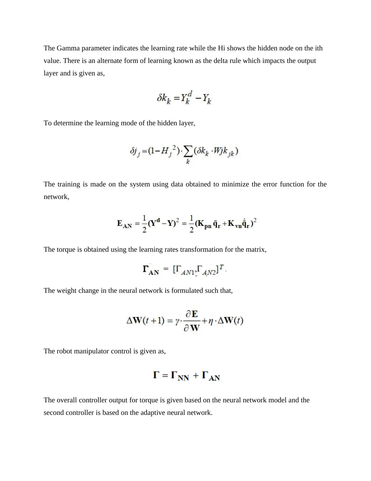
The Gamma parameter indicates the learning rate while the Hi shows the hidden node on the ith
value. There is an alternate form of learning known as the delta rule which impacts the output
layer and is given as,
To determine the learning mode of the hidden layer,
The training is made on the system using data obtained to minimize the error function for the
network,
The torque is obtained using the learning rates transformation for the matrix,
The weight change in the neural network is formulated such that,
The robot manipulator control is given as,
The overall controller output for torque is given based on the neural network model and the
second controller is based on the adaptive neural network.
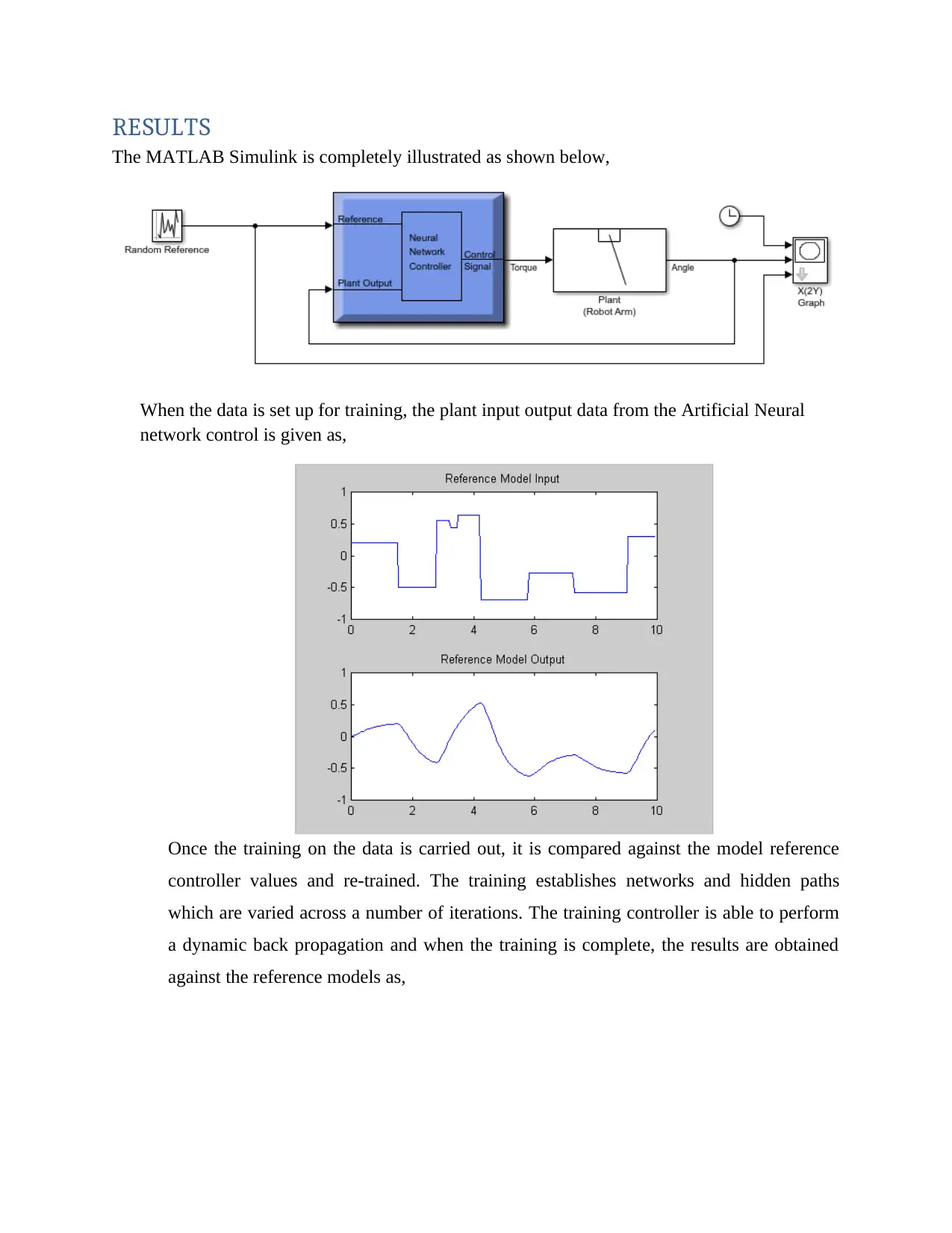
RESULTS
The MATLAB Simulink is completely illustrated as shown below,
When the data is set up for training, the plant input output data from the Artificial Neural
network control is given as,
Once the training on the data is carried out, it is compared against the model reference
controller values and re-trained. The training establishes networks and hidden paths
which are varied across a number of iterations. The training controller is able to perform
a dynamic back propagation and when the training is complete, the results are obtained
against the reference models as,
⊘ This is a preview!⊘
Do you want full access?
Subscribe today to unlock all pages.
Trusted by 1+ million students worldwide
1 out of 17

Your All-in-One AI-Powered Toolkit for Academic Success.
+13062052269
info@desklib.com
Available 24*7 on WhatsApp / Email
![[object Object]](/_next/static/media/star-bottom.7253800d.svg)
Unlock your academic potential
Copyright © 2020–2026 A2Z Services. All Rights Reserved. Developed and managed by ZUCOL.