300596 Advanced Signal Processing Project: Tone Detection Report

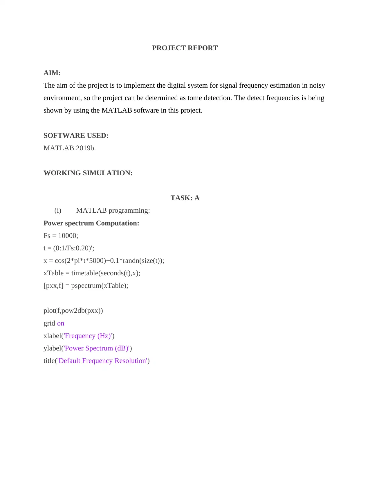
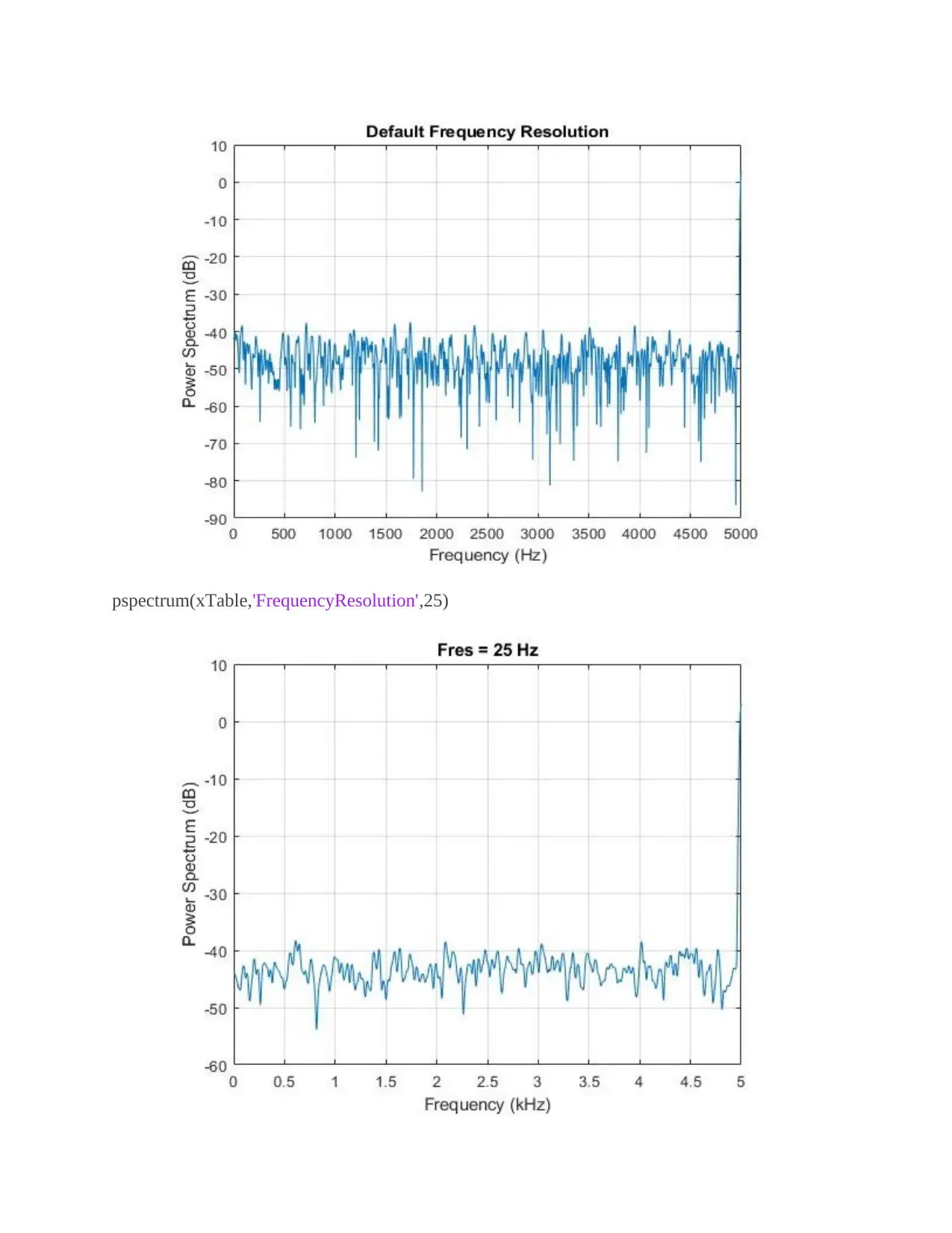
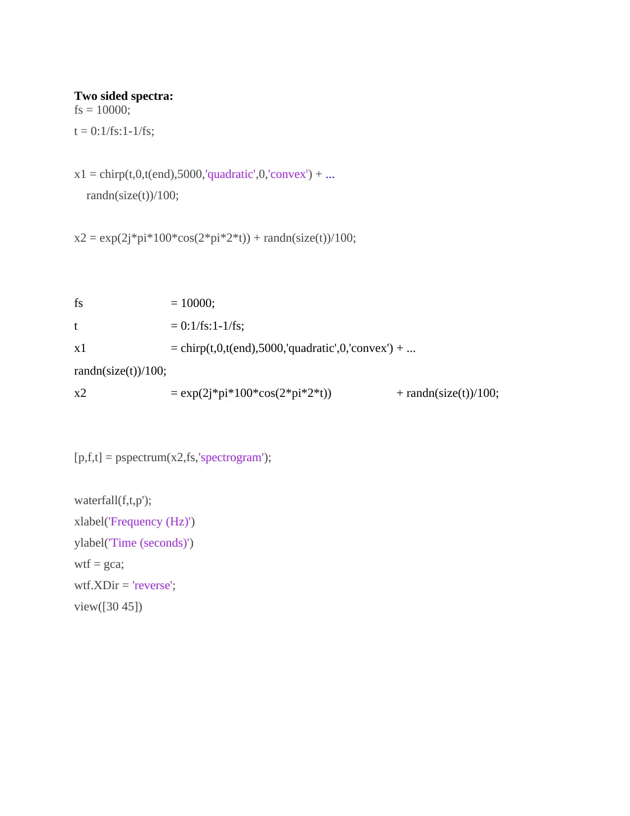
This project report details the implementation of a digital system for signal frequency estimation in a noisy environment, also known as tone detection. The project utilizes MATLAB software to analyze and visualize the detected frequencies. The report includes code and explanations for power spectrum computation, two-sided spectra, window leakage and tone resolution, and the persistence spectrum of transient signals. The report also includes an additional task focusing on spectrogram and reassigned spectrogram analysis of a chirp signal. The student successfully computed and visualized spectrogram parameters, including generation of a quadratic chirp and reassigned spectrograms at different time and frequency resolutions. The analysis covers various aspects of signal processing, including frequency determination, harmonics, and the challenges of working with noisy signals. The project aims to provide a practical understanding of signal processing techniques and their application in real-world scenarios.

300596 Advanced Signal Processing
Project
TONE DETECTION

PROJECT REPORT
AIM:
The aim of the project is to implement the digital system for signal frequency estimation in noisy
environment, so the project can be determined as tome detection. The detect frequencies is being
shown by using the MATLAB software in this project.
SOFTWARE USED:
MATLAB 2019b.
WORKING SIMULATION:
TASK: A
(i) MATLAB programming:
Power spectrum Computation:
Fs = 10000;
t = (0:1/Fs:0.20)';
x = cos(2*pi*t*5000)+0.1*randn(size(t));
xTable = timetable(seconds(t),x);
[pxx,f] = pspectrum(xTable);
plot(f,pow2db(pxx))
grid on
xlabel('Frequency (Hz)')
ylabel('Power Spectrum (dB)')
title('Default Frequency Resolution')

pspectrum(xTable,'FrequencyResolution',25)

Two sided spectra:
fs = 10000;
t = 0:1/fs:1-1/fs;
x1 = chirp(t,0,t(end),5000,'quadratic',0,'convex') + ...
randn(size(t))/100;
x2 = exp(2j*pi*100*cos(2*pi*2*t)) + randn(size(t))/100;
fs = 10000;
t = 0:1/fs:1-1/fs;
x1 = chirp(t,0,t(end),5000,'quadratic',0,'convex') + ...
randn(size(t))/100;
x2 = exp(2j*pi*100*cos(2*pi*2*t)) + randn(size(t))/100;
[p,f,t] = pspectrum(x2,fs,'spectrogram');
waterfall(f,t,p');
xlabel('Frequency (Hz)')
ylabel('Time (seconds)')
wtf = gca;
wtf.XDir = 'reverse';
view([30 45])

Window Leakage and Tone Resolution:
fs = 10000;
t = (0:1/fs:2-1/fs)';
x = sin(2*pi*[0 5000].*t) + [1 1/100].*sin(2*pi*[0 5000].*t);
x = x + randn(size(x)).*std(x)/db2mag(40);
plot(t,x)

pspectrum(x,t)
pspectrum(x,t,'Leakage',0.85)
Persistence Spectrum of Transient Signal

fs = 10000;
t = (0:1/fs:500)';
x = chirp(t,0,t(end),3000) + 0.15*randn(size(t));
idx = floor(length(x)/6);
x(1:idx) = x(1:idx) + 0.05*cos(2*pi*t(1:idx)*210);
pspectrum(x,fs,'spectrogram', ...
'FrequencyLimits',[100 290],'TimeResolution',1)
pspectrum(x,fs,'FrequencyLimits',[100 290])

pspectrum(x,fs,'persistence', ...
'FrequencyLimits',[100 290],'TimeResolution',1)

(ii) Program Explanation:
For power spectrum computation:
Computation of the power spectrum for a noisy sinusoid is being shown below. For this
computation, sinusoidal frequency should be specified at 5000Hz. And its sampling frequency
should be 10000Hz for the time value at 20ms. After this simulation the signal can be embedded
with the white Gaussian noise which is having the value for variance as 0.1.
Then the re-computation of the sinusoid power spectrum can be done, where the frequency
resolution will be at 25Hz. Then the plotting of the spectrum for pspectrum function without
output arguments will be done.
For Two- sided Spectra:
Two signal generations will be done with sampling of each frequency at 10000Hz for the time at
1 sec. In which the first signal can be determined as the convex quadratic chirp, which will have
the frequency variation of 0-5000Hz at the time of measurement. This chirp signal will be
merged with the white Gaussian noise.

For Window Leakage and Tone Resolution:
Generate a two-channel signal sampled at 10000 Hz for 2 seconds.
1. The first channel consists of a 0-5000Hz tone. Both tones have unit amplitude.
2. The second channel also has two tones. One tone has unit amplitude and a frequency of 20
Hz. The other tone has amplitude of 1/100 and a frequency of 30 Hz.
Embed the signal in white noise. Specify a signal-to-noise ratio of 40 dB. Plot the signals.
For Persistence Spectrum of Transient Signal:
Visualize an interference narrowband signal embedded within a broadband signal.
Generate a chirp sampled at 10000 Hz for 500 seconds. The frequency of the chirp increases
from 0 Hz to 5000 Hz during the measurement.
The signal also contains a 210 Hz sinusoid. The sinusoid has amplitude of 0.05 and is present
only for 1/6 of the total signal duration.
Compute the spectrogram of the signal. Restrict the frequency range from 100 Hz to 290 Hz.
Specify a time resolution of 1 second. Both signal components are visible.
Compute the power spectrum of the signal. The weak sinusoid is obscured by the chirp.
Compute the persistence spectrum of the signal. Now both signal components are clearly visible.
(iii) 15 tones Frequencies list in chronological order
Comparison with
fundamentals
Tone Interval Frequency ratio Tone Frequency(Hz)
Fundamental
Frequency fundamental
1:1 C 65
Double
Frequency octave
2:1 c 130
Trifold
frequency
Fifth 3:2 g 195
Fourfold
frequency fourth
4:3 c’ 260

Fivefold
frequency major third
5:4 e’ 325
Six fold
frequency minor third
6:5 g’ 390
Sevenfold
frequency
7:6 Natural seventh 455
Eightfold
frequency
8:7 c’’ 520
Nine fold
frequency large whole tone
9:8 d’’ 585
Tenfold
frequency small whole tone
10:9 e’’ 650
Eleven fold
frequency
11:10 Alphorn F-5 715
Twelvefold
frequency
12:11 g’’ 780
Thirteen fold
frequency
13:12 845
Fourteen fold
frequency
14:13 b’’ 910
Fifteen fold
frequency
15:14 c’’’ 975
(iv) Frequency Determination:
Overtone can be determined as (Harmonics-1),
Or Harmonics can be determined as (Overtones + 1)
For a certain frequency, there are some integer multiples, which is known as Harmonics, Partials
or the overtones. In which overtone doesn’t include the fundamental frequency. The first
overtone already exists as second harmonic. The overtone cannot be mixed with another term as
it has the unequal counting. The term harmonic can be determined as the fundamental frequency
multiple for a vibrating object.

TASK B: Additional task
a. Aim of the Task:
The aim of the additional task is Spectrogram and Reassigned Spectrogram of Chirp and
computation of reassigned spectrogram by specified a frequency resolution. And provide the
generation of quadratic chirp samples.
b. Purpose of Additional Task:
By this project’s additional task it would be possible to provide the computation of spectrogram by using
the pspectrum function default setting.
c. Challenges of this task as compare to Part A:
The main challenge of this additional task is that, without using the parameters from the task A it is not
possible to complete the additional task. So it is important to perform task A before providing the
computation of spectrogram.
d. Procedure for doing the task:
This additional task is being done by using the MATLAB software by doing all the computation through
MATLAB coding. The procedure and coding is being given below:
Spectrogram and Reassigned Spectrogram of Chirp:
The MATLAB coding given below generates a quadratic chirp, which is being sampled at 1KHz
for the time of 2 seconds. The chirp frequency should have the initial frequency of 100 Hz
which will increase up to 200Hz for the time at t=1 sec. so the computation of spectrogram using
the pspectrum function default setting is being shown below:
fs = 1e3;
t = 0:1/fs:2;
y = chirp(t,100,1,200,'quadratic');
[sp,fp,tp] = pspectrum(y,fs,'spectrogram');