Numerical Analysis of Thermal and Fluid Engineering Project, 301023

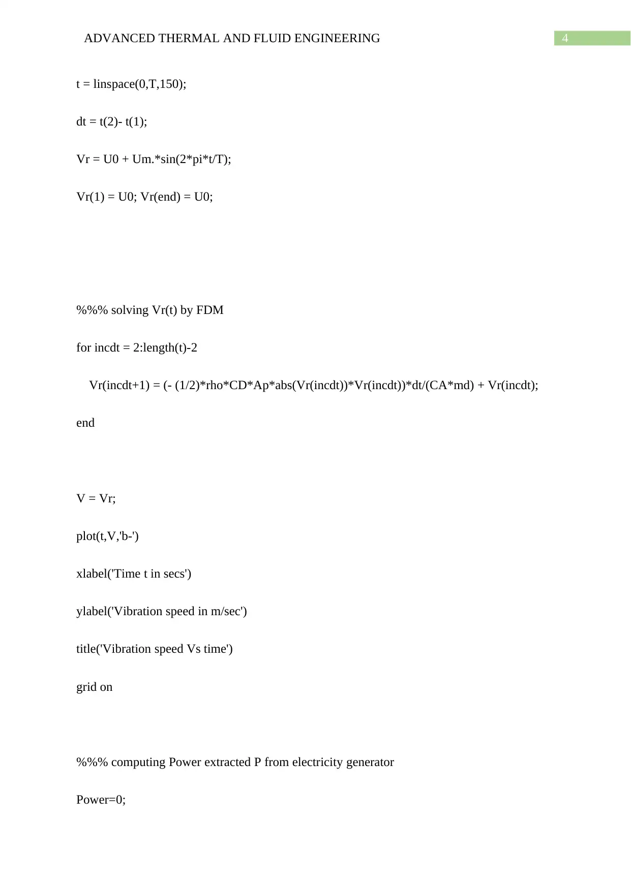
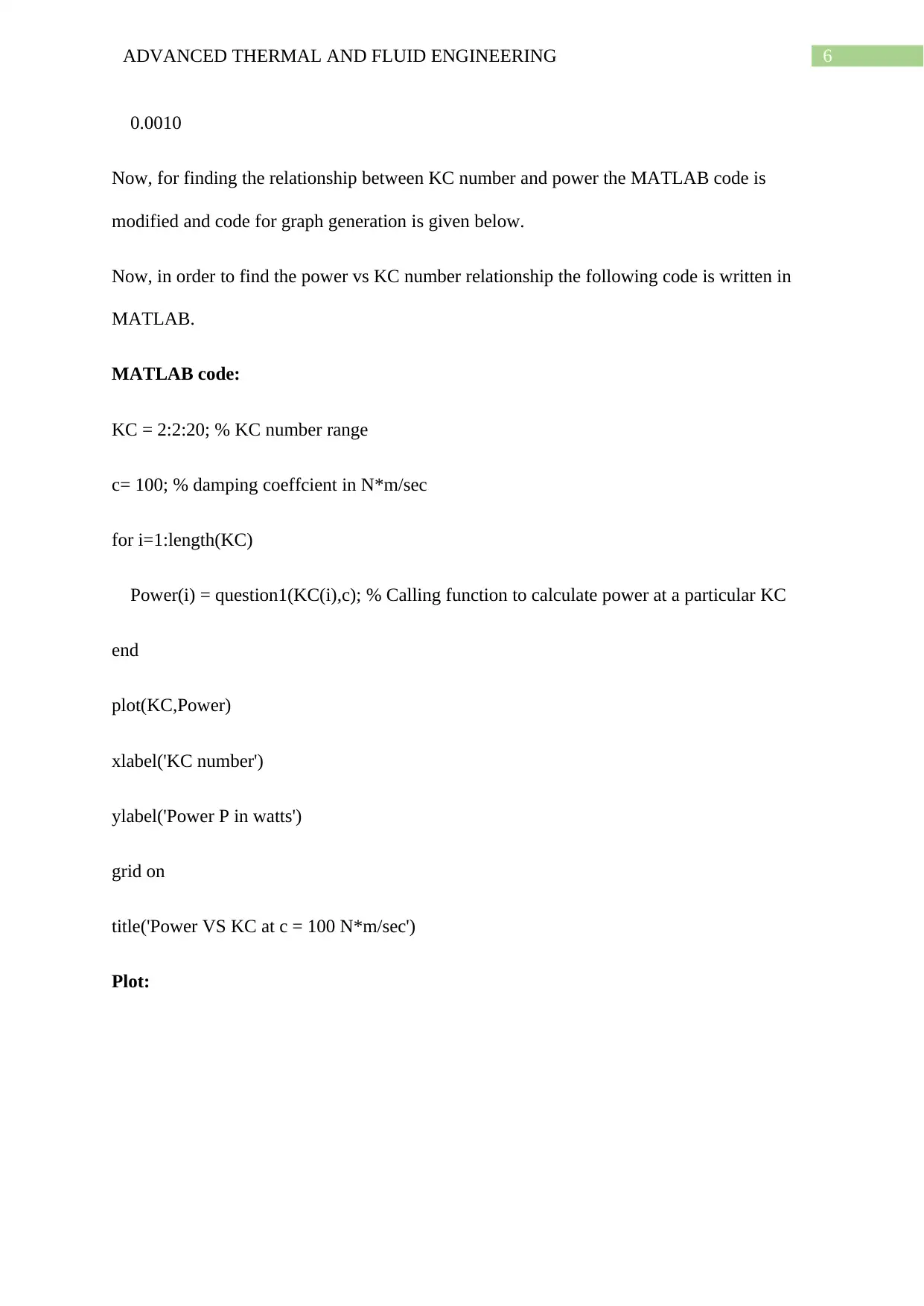
This project presents a comprehensive analysis of advanced thermal and fluid engineering concepts through two distinct parts. The first part focuses on modeling the equation of motion for a cylinder with variable water flow and determining its vibration using a Finite Difference Method (FDM) approach. This section includes deriving the equation of motion, developing a numerical method, and providing MATLAB code to simulate the vibration speed and calculate the extracted power, along with graphs illustrating the relationships between KC number, damping coefficient, and power. The second part explores a one-dimensional convection-diffusion problem, utilizing FDM to solve a 2-D heat equation describing soil heating by groundwater flow. This part includes deriving the governing equation, applying boundary conditions, and providing MATLAB code to calculate and plot temperature variations over time and depth, as well as analyzing the effect of the heat diffusion coefficient on temperature profiles. The project aims to provide a practical understanding of numerical methods in thermal and fluid engineering.

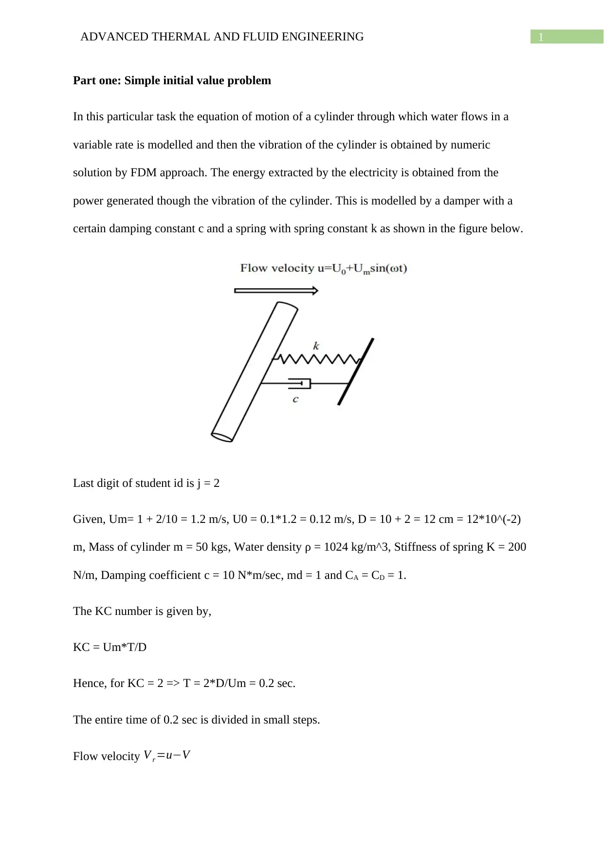
Running head: ADVANCED THERMAL AND FLUID ENGINEERING
ADVANCED THERMAL AND FLUID ENGINEERING
Name of the Student
Name of the University
Author Note

1ADVANCED THERMAL AND FLUID ENGINEERING
Part one: Simple initial value problem
In this particular task the equation of motion of a cylinder through which water flows in a
variable rate is modelled and then the vibration of the cylinder is obtained by numeric
solution by FDM approach. The energy extracted by the electricity is obtained from the
power generated though the vibration of the cylinder. This is modelled by a damper with a
certain damping constant c and a spring with spring constant k as shown in the figure below.
Last digit of student id is j = 2
Given, Um= 1 + 2/10 = 1.2 m/s, U0 = 0.1*1.2 = 0.12 m/s, D = 10 + 2 = 12 cm = 12*10^(-2)
m, Mass of cylinder m = 50 kgs, Water density ρ = 1024 kg/m^3, Stiffness of spring K = 200
N/m, Damping coefficient c = 10 N*m/sec, md = 1 and CA = CD = 1.
The KC number is given by,
KC = Um*T/D
Hence, for KC = 2 => T = 2*D/Um = 0.2 sec.
The entire time of 0.2 sec is divided in small steps.
Flow velocity V r =u−V

2ADVANCED THERMAL AND FLUID ENGINEERING
Now, initially, V r (0) = V(0) = U0 and V r (end) = U0
Now, the Morrison equation is given by,
Fwater=C A∗md∗( d V r
dt )+ ( ½ )∗ρ∗CD∗A P∗|V r |∗V r
Now, value of Fwater will be => mass of water*g = 1024*(2*pi*D/2)*L*9.8 = 5990 N.
The Morrison equation by finite difference approximation is given as,
CA∗md∗Vr ( t +dt ) −Vr ( t )
dt + ( ½ )∗ρ∗CD∗AP∗|V r ( t )|∗V r ( t ) =0
 Vr ( t +dt )= (− ( ½ )∗ρ∗CD∗A P∗|V r ( t )|∗V r ( t ) ) dt
CA∗md
+Vr ( t )
From V r (t+dt ) Obtained from the above iteration equation, V(t) can be easily obtained for
each points in the time range [0,T].
The discrete numerical integration relation that gives approximate power P is given by,
P = 1
N ∑
n=1
N
c∗(V ¿¿ n)2 ¿
N = total number by which T is divided.
MATLAB code for Vibration speed:
function Power = question1(KC,c)
j = 2;
%%% defining parameters of the system
% amplitude of oscillatory flow in m/s
Um = 1 + (j/10);

3ADVANCED THERMAL AND FLUID ENGINEERING
% steady state flow in m/s
U0 = 0.1*Um;
% diameter in m
D = (10 + j)*1e-2;
% length of the cylinder
L = 1;
% mass of cylinder
m = 50;
% density of the water in Kg/m^3
rho = 1024;
% spring stiffness N/m
K = 200;
% the surface of the cylinder is the projected area
Ap = 2*pi*(D/2)*L;
% added mass coefficient
md = 1;
CA = 1.8; CD = 1.8; T = KC*D/Um;
Fwater = 1024*(2*pi*D/2)*L*9.8;

4ADVANCED THERMAL AND FLUID ENGINEERING
t = linspace(0,T,150);
dt = t(2)- t(1);
Vr = U0 + Um.*sin(2*pi*t/T);
Vr(1) = U0; Vr(end) = U0;
%%% solving Vr(t) by FDM
for incdt = 2:length(t)-2
Vr(incdt+1) = (- (1/2)*rho*CD*Ap*abs(Vr(incdt))*Vr(incdt))*dt/(CA*md) + Vr(incdt);
end
V = Vr;
plot(t,V,'b-')
xlabel('Time t in secs')
ylabel('Vibration speed in m/sec')
title('Vibration speed Vs time')
grid on
%%% computing Power extracted P from electricity generator
Power=0;

5ADVANCED THERMAL AND FLUID ENGINEERING
for i=1:length(t)
Power = Power + c*(abs(V(i))^i)^2;
end
Power = Power/length(t);
%fprintf('The total power P extracted from generator for KC number =2 is %.3f Watts',P)
end
Output:
0 0.02 0.04 0.06 0.08 0.1 0.12 0.14 0.16 0.18 0.2
Time t in secs
0.02
0.04
0.06
0.08
0.1
0.12
0.14
0.16
0.18
Vibration speed in m/sec
Vibration speed Vs time
The total power P extracted from generator for KC number =2 is 0.001 Watts
Power =

6ADVANCED THERMAL AND FLUID ENGINEERING
0.0010
Now, for finding the relationship between KC number and power the MATLAB code is
modified and code for graph generation is given below.
Now, in order to find the power vs KC number relationship the following code is written in
MATLAB.
MATLAB code:
KC = 2:2:20; % KC number range
c= 100; % damping coeffcient in N*m/sec
for i=1:length(KC)
Power(i) = question1(KC(i),c); % Calling function to calculate power at a particular KC
end
plot(KC,Power)
xlabel('KC number')
ylabel('Power P in watts')
grid on
title('Power VS KC at c = 100 N*m/sec')
Plot:

7ADVANCED THERMAL AND FLUID ENGINEERING
2 4 6 8 10 12 14 16 18 20
KC number
0.010164
0.010166
0.010168
0.01017
0.010172
0.010174
0.010176
0.010178
Power P in watts
Power VS KC at c = 100 N*m/sec
It can be seen from the above graph that as the KC number is increased the power extracted
has been decreased this is because KC number is inversely proportional to the power.
Now, KC number is kept constant at 10 and value of c is varied in the range 0 to 2000
N*m/sec by step of 50.
MATLAB code:
KC = 10; % fized KC number
c = 0:50:2000; % variable damping coeffcient
for i=1:length(c)
Power(i) = question1(KC,c(i)); % Power at different coeffcient
end
plot(c,Power)

8ADVANCED THERMAL AND FLUID ENGINEERING
xlabel('Damping coefcient c in N*m/sec')
ylabel('Power in watts')
grid on
title('Power VS damping coeffcient at KC = 10')
Output:
0 200 400 600 800 1000 1200 1400 1600 1800 2000
Damping coefcient c in N*m/sec
0
0.05
0.1
0.15
0.2
0.25
Power in watts
Power VS damping coeffcient at KC = 10
A linear relationship can be observed from the graph as the extracted power from generator is
directly proportional to the damping coefficient.
Part two: One-dimensional convection diffusion problem
The last digit of student ID is j = 2
The finite difference method is applied to solve the 2-D heat equation described by the
following picture.

9ADVANCED THERMAL AND FLUID ENGINEERING
The ground water flows through the pores of the soli and gradually the hot water warms the
soil. The objective is to obtained heating behaviour of the soil with time up to a depth of x=2
meters from surface. Initially the entire volume of the water is at 10 + 2 = 12 °C. The surface
that just touching the water level is maintained at 30 °C.
The x length is the length taken from the surface to 2 meters depth. The heat governing
equation is given by,
T
t =−u∗( T
x )+ α∗❑2 T
x2 (1)
T = soil temperature as a function of x and t = T(x,t)
t = time in secs.
u = water flow velocity = 0.002*(1+2) = 0.002*3= 0.006 m/s.
α = heat diffusion coefficient with consideration of soil influence = 0.0002 m^2/sec.
x=0 to x=2 meters is subdivided in 200 points.

10ADVANCED THERMAL AND FLUID ENGINEERING
x= 0 = 1st cell and
x= 2 = 200th cell.
Hence, by finite difference approximation the differential equation (1) becomes
T ( x , t +1 ) – T ( x ,t )
dt =−u∗T ( x +1 , t ) – T ( x , t )
dx + α∗T ( x +1 ,t ) – 2∗T ( x , t ) + T ( x−1 ,t )
d x2
OR,
T ( x , t+1 ) = ( −u∗T ( x+1 , t ) – T ( x , t )
dx + α∗T ( x +1 , t ) – 2∗T ( x ,t ) +T ( x−1 , t )
d x2 )∗dt +T (x , t)
Variation of temperature = i-1 to i+1 cells
Where, i-1 to i+1 varies from temperature at 1st to 200th cell or point.
Boundary conditions are T|x=0 = 30 °C, T
x =0 at x= 2.
Also, T(i) = (10 + j) = (10+2) °C = 12 °C initially.
T
x =0 at x= 2 => (T(200,t) – T(199,t))/dx = 0
Hence, T(200,t) = T(199,t) Or, T(200,t) = T(199,t)
Hence, by finite difference method temperatures from T(1) to T(199) is calculated and then
the value of T(199) is made equal to T(200).
MATLAB code for temperature plot and T1.5 at α = 0.0002 m^2/sec:
function time25 = question2(alpha) % coeffcient of heat diffusion in m^2/sec
j=2;
% flow velocity

11ADVANCED THERMAL AND FLUID ENGINEERING
u = 0.002*(1+j);
% dividing 0 to 2 meters
x= linspace(0,2,200);
% step increment of x
dx = x(2) - x(1);
% unit increment of time
dt = 2*dx;
% 0 to 300 secs
t = 0:dt:300;
% initial temperature is 12 degree C
initialT = 10+j;
% initially T is at 12 degree C for all t and x
Temp = repmat(initialT,length(x),length(t));
% applying boundary conditions
Temp(1,:) = 30; Temp(199,:) = Temp(200,:);
for incdt = 1:length(t)-1
for incdx = 2:length(x)-1