Evaluating Share Price Behavior of AGL Energy Limited (AGL.AX)

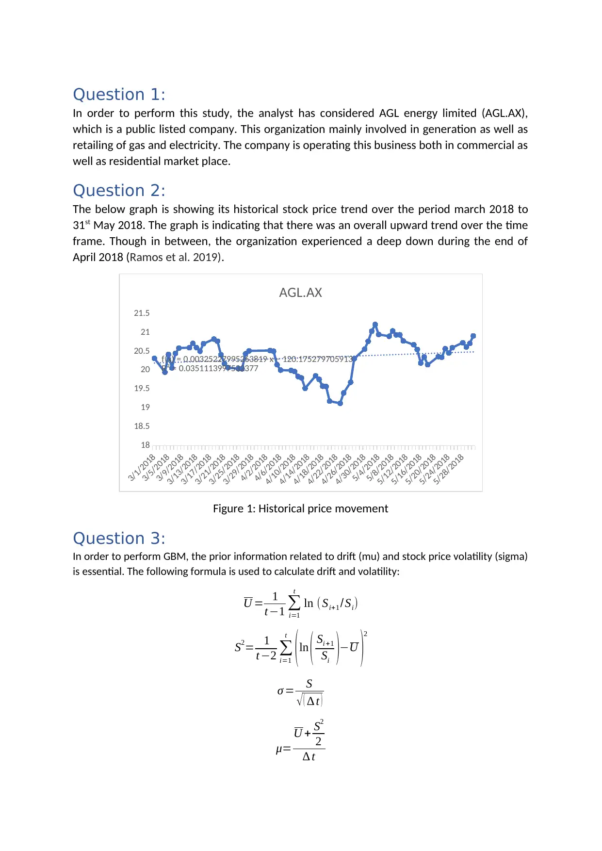
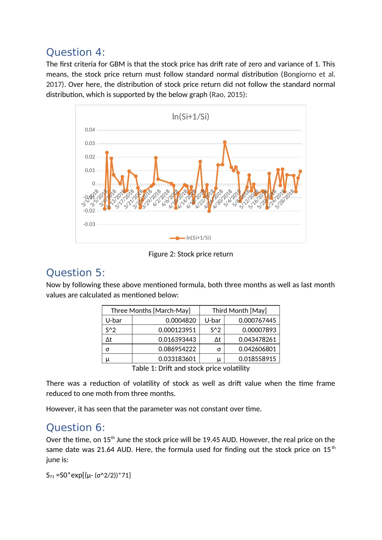
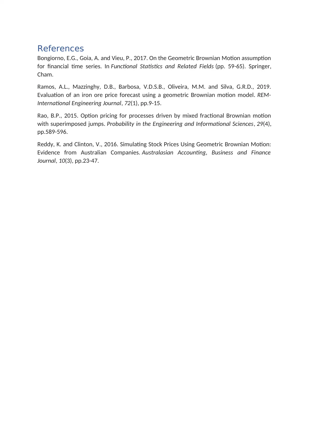
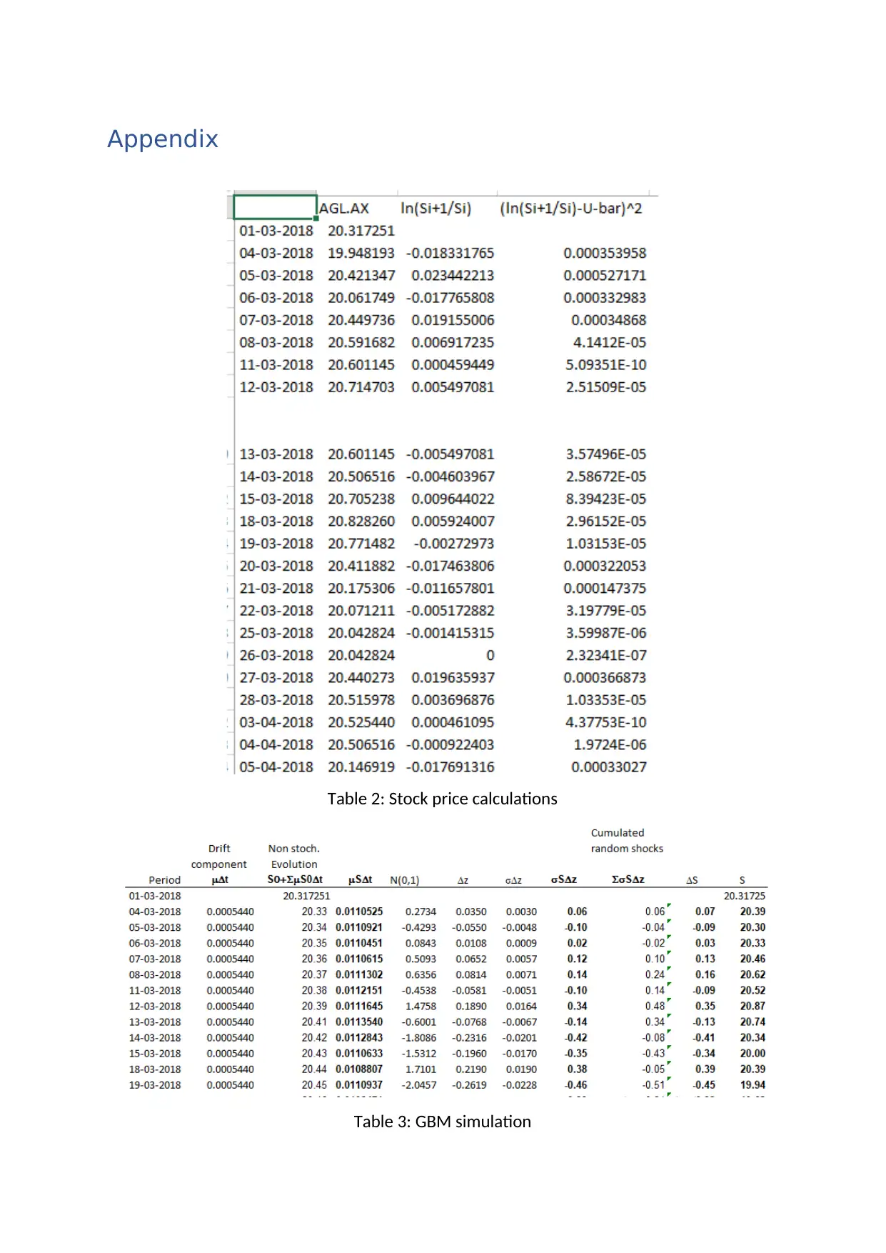
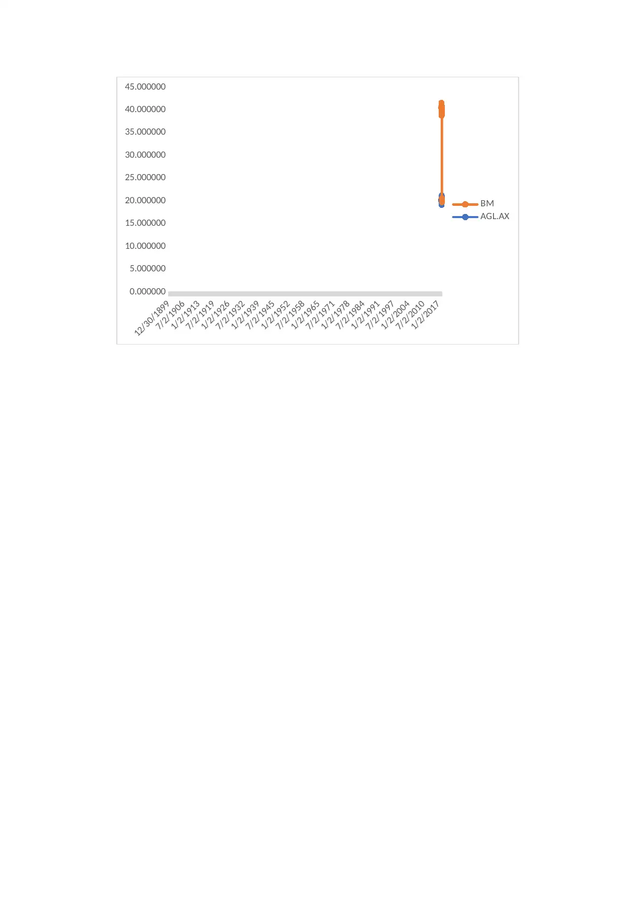
This report examines the behavior and performance of AGL Energy Limited's (AGL.AX) share price, utilizing the geometric Brownian motion (GBM) model. The analysis covers the period from March to May 2018, revealing an overall upward trend with a significant dip in late April. The study calculates drift and volatility using historical stock prices, noting that the stock price return does not strictly follow a standard normal distribution, a key criterion for GBM. Volatility and drift values are computed for both a three-month and a one-month period, showing a reduction in these parameters when the timeframe is shortened. A prediction of the stock price on June 15th is made using the GBM model and compared to the actual price, revealing a discrepancy. The report references academic works discussing the application and limitations of GBM in simulating stock price movements. Desklib offers a variety of study tools, including solved assignments and past papers, to aid students in their academic pursuits.

Behavior and Performance of Share Price
Name of the Student
Name of the University

Table of Contents
Question 1:............................................................................................................................................3
Question 2:............................................................................................................................................3
Question 3:............................................................................................................................................3
Question 4:............................................................................................................................................4
Question 5:............................................................................................................................................4
Question 6:............................................................................................................................................4
Question 7:............................................................................................................................................4
References.............................................................................................................................................5
Appendix...............................................................................................................................................6

Question 1:
In order to perform this study, the analyst has considered AGL energy limited (AGL.AX),
which is a public listed company. This organization mainly involved in generation as well as
retailing of gas and electricity. The company is operating this business both in commercial as
well as residential market place.
Question 2:
The below graph is showing its historical stock price trend over the period march 2018 to
31st May 2018. The graph is indicating that there was an overall upward trend over the time
frame. Though in between, the organization experienced a deep down during the end of
April 2018 (Ramos et al. 2019).
3/1/2018
3/5/2018
3/9/2018
3/13/2018
3/17/2018
3/21/2018
3/25/2018
3/29/2018
4/2/2018
4/6/2018
4/10/2018
4/14/2018
4/18/2018
4/22/2018
4/26/2018
4/30/2018
5/4/2018
5/8/2018
5/12/2018
5/16/2018
5/20/2018
5/24/2018
5/28/2018
18
18.5
19
19.5
20
20.5
21
21.5
f(x) = 0.00325227995263819 x − 120.175279705913
R² = 0.0351113997532377
AGL.AX
Figure 1: Historical price movement
Question 3:
In order to perform GBM, the prior information related to drift (mu) and stock price volatility (sigma)
is essential. The following formula is used to calculate drift and volatility:
U = 1
t−1 ∑
i=1
t
ln ( Si+1 /Si)
S2= 1
t −2 ∑
i=1
t
( ln ( Si +1
Si )−U )
2
σ = S
√ ( ∆ t )
μ=
U + S2
2
∆ t

Question 4:
The first criteria for GBM is that the stock price has drift rate of zero and variance of 1. This
means, the stock price return must follow standard normal distribution (Bongiorno et al.
2017). Over here, the distribution of stock price return did not follow the standard normal
distribution, which is supported by the below graph (Rao, 2015):
3/1/2018
3/5/2018
3/9/2018
3/13/2018
3/17/2018
3/21/2018
3/25/2018
3/29/2018
4/2/2018
4/6/2018
4/10/2018
4/14/2018
4/18/2018
4/22/2018
4/26/2018
4/30/2018
5/4/2018
5/8/2018
5/12/2018
5/16/2018
5/20/2018
5/24/2018
5/28/2018
-0.03
-0.02
-0.01
0
0.01
0.02
0.03
0.04
ln(Si+1/Si)
ln(Si+1/Si)
Figure 2: Stock price return
Question 5:
Now by following these above mentioned formula, both three months as well as last month
values are calculated as mentioned below:
Three Months [March-May] Third Month [May]
U-bar 0.0004820 U-bar 0.000767445
S^2 0.000123951 S^2 0.00007893
∆t 0.016393443 ∆t 0.043478261
σ 0.086954222 σ 0.042606801
μ 0.033183601 μ 0.018558915
Table 1: Drift and stock price volatility
There was a reduction of volatility of stock as well as drift value when the time frame
reduced to one moth from three months.
However, it has seen that the parameter was not constant over time.
Question 6:
Over the time, on 15th June the stock price will be 19.45 AUD. However, the real price on the
same date was 21.64 AUD. Here, the formula used for finding out the stock price on 15 th
june is:
S71 =S0*exp[(μ- (σ^2/2))*71]

Question 7:
It has seen that the study of the geometric Brownian motion (GBM) method to simulate stock price
movements and do prediction implies whether the simulated stock prices align with actual stock
returns (Reddy and Clinton, 2016).

References
Bongiorno, E.G., Goia, A. and Vieu, P., 2017. On the Geometric Brownian Motion assumption
for financial time series. In Functional Statistics and Related Fields (pp. 59-65). Springer,
Cham.
Ramos, A.L., Mazzinghy, D.B., Barbosa, V.D.S.B., Oliveira, M.M. and Silva, G.R.D., 2019.
Evaluation of an iron ore price forecast using a geometric Brownian motion model. REM-
International Engineering Journal, 72(1), pp.9-15.
Rao, B.P., 2015. Option pricing for processes driven by mixed fractional Brownian motion
with superimposed jumps. Probability in the Engineering and Informational Sciences, 29(4),
pp.589-596.
Reddy, K. and Clinton, V., 2016. Simulating Stock Prices Using Geometric Brownian Motion:
Evidence from Australian Companies. Australasian Accounting, Business and Finance
Journal, 10(3), pp.23-47.

Appendix
Table 2: Stock price calculations
Table 3: GBM simulation

12/30/1899
7/2/1906
1/2/1913
7/2/1919
1/2/1926
7/2/1932
1/2/1939
7/2/1945
1/2/1952
7/2/1958
1/2/1965
7/2/1971
1/2/1978
7/2/1984
1/2/1991
7/2/1997
1/2/2004
7/2/2010
1/2/2017
0.000000
5.000000
10.000000
15.000000
20.000000
25.000000
30.000000
35.000000
40.000000
45.000000
BM
AGL.AX