BUS708 Statistics: Statistical Modeling of Airline Data Analysis
VerifiedAdded on 2023/04/25
|11
|2460
|55
Report
AI Summary
This report analyzes two datasets related to airline services in Australia to provide recommendations for improving airport services, particularly at Sydney Airport. The analysis involves exploring flight data from 2003 to 2018, identifying key variables, and forming hypotheses. Statistical methods such as histograms, z-tests, and ANOVA are used to analyze single and multiple variables, focusing on factors like airlines, Australian cities, and flight counts. The findings indicate that Sydney Airport has the highest flight activity compared to Melbourne and Brisbane. The report concludes that Sydney's prominence may be due to tourist preferences and airline choices, influencing the airport's flight volume. Desklib provides access to this report and other study tools.
Section 1: Introduction
a)
(Minton, 2018)
b) This dataset is a primary data where no statistical method has been applied to modify the
dataset. The data gives the information of different flights which run between Australia and
different international cities in the world in the different months of the year for a period of
15 years from 2003 to 2018. The record is keeping track of how many flights are leaving the
country and how many are coming in which indirectly will give a count of people travelling
across different countries.
The variables involved are:
Variable Description Values
In-Out Airlines comes in or
goes out
I for in and O for out
Australian City Which Australian city
airline lands or Flies
out.
Australian city names
International City Which international
city airline lands or
flies out
International city
names
Airlines Name of the airline Name of the airline
Route Via which airport
airlines flies
Short forms of various
airports
Port country Which country airlines
belongs to
Name of the country
Port Region Which region airline
belongs
Region name
Service country Which country do the
service
Country name
Stops Number of stops
airlines have
0,1,2
All Flights Number flight in or out Number in integer
Paraphrase This Document
Need a fresh take? Get an instant paraphrase of this document with our AI Paraphraser
in the month
Max seat Number of maximum
seats
Number in integer
Year Which year Number in the year
Month Number Which month Number of the month
From the list of variables we can think few variables which will have an impact. So we can consider
the column All Flights as the response variable and Max seat, Month Number, Stops, Airlines, Routes
are some of the independent variables that we can think of
i) The most important case that can be considered is that which airlines have the all flight
count maximum or else all flight counts depends on the airlines.
ii) Also we can think that how can number of stops affect the all flight.
iii) Whether the maximum number of seats is also one of the factor for determining the
type of airlines and as we have mentioned in 1st case that the type of airlines affects the
all flights concept so indirectly we can say that maximum number of seats is affecting
the variable all flights.
c) We have picked a random sample of 1000 from the initial dataset1. Yes it is a secondary
dataset as we have processed the data.
From the list of variables we can think few variables which will have an impact. So we can consider
the column All Flights as the response variable and Max seat, Month Number, Stops, Airlines, Routes
are some of the independent variables that we can think of.
i) The most important case that can be considered is that which airlines have the all flight
count maximum or else all flight counts depends on the airlines.
ii) Also we can think that how can number of stops affect the all flight.
iii) Whether the maximum number of seats is also one of the factor for determining the
type of airlines and as we have mentioned in 1st case that the type of airlines affects the
all flights concept so indirectly we can say that maximum number of seats is affecting
the variable all flights.
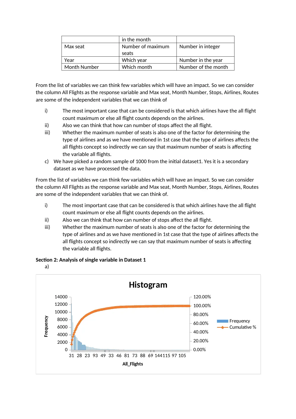
Section 2: Analysis of single variable in Dataset 1
a)
31 28 23 93 49 33 46 81 73 88 69 144115 97 105
0
2000
4000
6000
8000
10000
12000
14000
0.00%
20.00%
40.00%
60.00%
80.00%
100.00%
120.00%
Histogram
Frequency
Cumulative %
All_Flights
Frequency
Max seat Number of maximum
seats
Number in integer
Year Which year Number in the year
Month Number Which month Number of the month
From the list of variables we can think few variables which will have an impact. So we can consider
the column All Flights as the response variable and Max seat, Month Number, Stops, Airlines, Routes
are some of the independent variables that we can think of
i) The most important case that can be considered is that which airlines have the all flight
count maximum or else all flight counts depends on the airlines.
ii) Also we can think that how can number of stops affect the all flight.
iii) Whether the maximum number of seats is also one of the factor for determining the
type of airlines and as we have mentioned in 1st case that the type of airlines affects the
all flights concept so indirectly we can say that maximum number of seats is affecting
the variable all flights.
c) We have picked a random sample of 1000 from the initial dataset1. Yes it is a secondary
dataset as we have processed the data.
From the list of variables we can think few variables which will have an impact. So we can consider
the column All Flights as the response variable and Max seat, Month Number, Stops, Airlines, Routes
are some of the independent variables that we can think of.
i) The most important case that can be considered is that which airlines have the all flight
count maximum or else all flight counts depends on the airlines.
ii) Also we can think that how can number of stops affect the all flight.
iii) Whether the maximum number of seats is also one of the factor for determining the
type of airlines and as we have mentioned in 1st case that the type of airlines affects the
all flights concept so indirectly we can say that maximum number of seats is affecting
the variable all flights.
Section 2: Analysis of single variable in Dataset 1
a)
31 28 23 93 49 33 46 81 73 88 69 144115 97 105
0
2000
4000
6000
8000
10000
12000
14000
0.00%
20.00%
40.00%
60.00%
80.00%
100.00%
120.00%
Histogram
Frequency
Cumulative %
All_Flights
Frequency
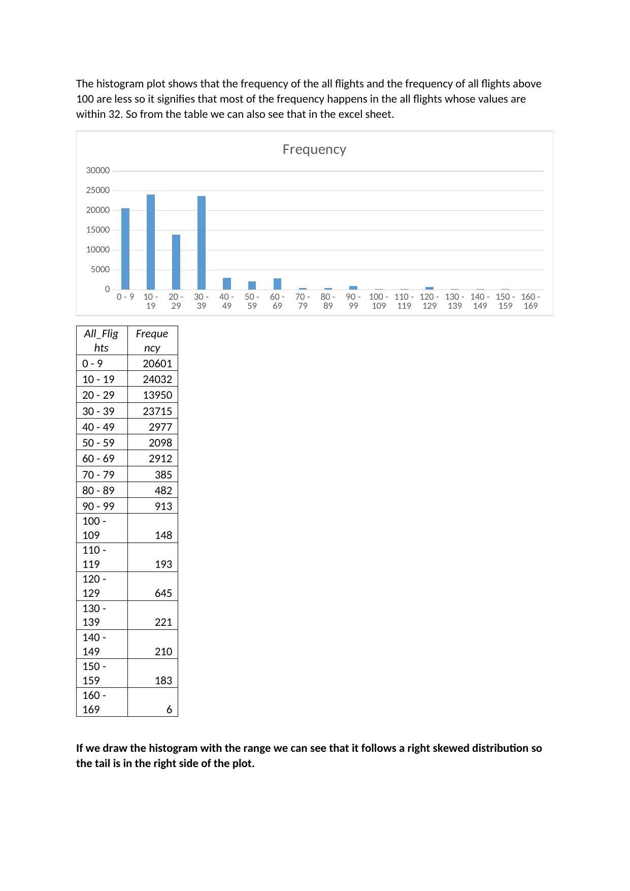
The histogram plot shows that the frequency of the all flights and the frequency of all flights above
100 are less so it signifies that most of the frequency happens in the all flights whose values are
within 32. So from the table we can also see that in the excel sheet.
0 - 9 10 -
19 20 -
29 30 -
39 40 -
49 50 -
59 60 -
69 70 -
79 80 -
89 90 -
99 100 -
109 110 -
119 120 -
129 130 -
139 140 -
149 150 -
159 160 -
169
0
5000
10000
15000
20000
25000
30000
Frequency
All_Flig
hts
Freque
ncy
0 - 9 20601
10 - 19 24032
20 - 29 13950
30 - 39 23715
40 - 49 2977
50 - 59 2098
60 - 69 2912
70 - 79 385
80 - 89 482
90 - 99 913
100 -
109 148
110 -
119 193
120 -
129 645
130 -
139 221
140 -
149 210
150 -
159 183
160 -
169 6
If we draw the histogram with the range we can see that it follows a right skewed distribution so
the tail is in the right side of the plot.
⊘ This is a preview!⊘
Do you want full access?
Subscribe today to unlock all pages.
Trusted by 1+ million students worldwide
0 - 19 20 - 39 40 - 59 60 - 79 80 - 99 100 - 119 120 - 139 140 - 159 160 - 179
0
5000
10000
15000
20000
25000
30000
35000
40000
45000
50000
Frequency
All_Flig
hts
Freque
ncy
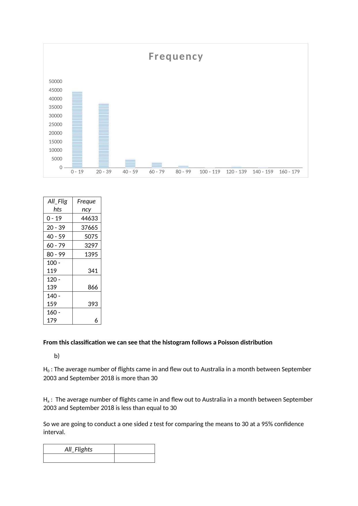
0 - 19 44633
20 - 39 37665
40 - 59 5075
60 - 79 3297
80 - 99 1395
100 -
119 341
120 -
139 866
140 -
159 393
160 -
179 6
From this classification we can see that the histogram follows a Poisson distribution
b)
H0 : The average number of flights came in and flew out to Australia in a month between September
2003 and September 2018 is more than 30
Ha : The average number of flights came in and flew out to Australia in a month between September
2003 and September 2018 is less than equal to 30
So we are going to conduct a one sided z test for comparing the means to 30 at a 95% confidence
interval.
All_Flights
0
5000
10000
15000
20000
25000
30000
35000
40000
45000
50000
Frequency
All_Flig
hts
Freque
ncy
0 - 19 44633
20 - 39 37665
40 - 59 5075
60 - 79 3297
80 - 99 1395
100 -
119 341
120 -
139 866
140 -
159 393
160 -
179 6
From this classification we can see that the histogram follows a Poisson distribution
b)
H0 : The average number of flights came in and flew out to Australia in a month between September
2003 and September 2018 is more than 30
Ha : The average number of flights came in and flew out to Australia in a month between September
2003 and September 2018 is less than equal to 30
So we are going to conduct a one sided z test for comparing the means to 30 at a 95% confidence
interval.
All_Flights
Paraphrase This Document
Need a fresh take? Get an instant paraphrase of this document with our AI Paraphraser
Mean
23.6867064
6
Standard Error
0.21614638
1
Median 19
Mode 30
Standard Deviation
20.7489268
2
Sample Variance
430.517964
1
Kurtosis
9.61666416
9
Skewness
2.56831007
3
Range 150
Minimum 0
Maximum 150
Sum 218273
Count 9215
Confidence
Level(95.0%) 0.42369478
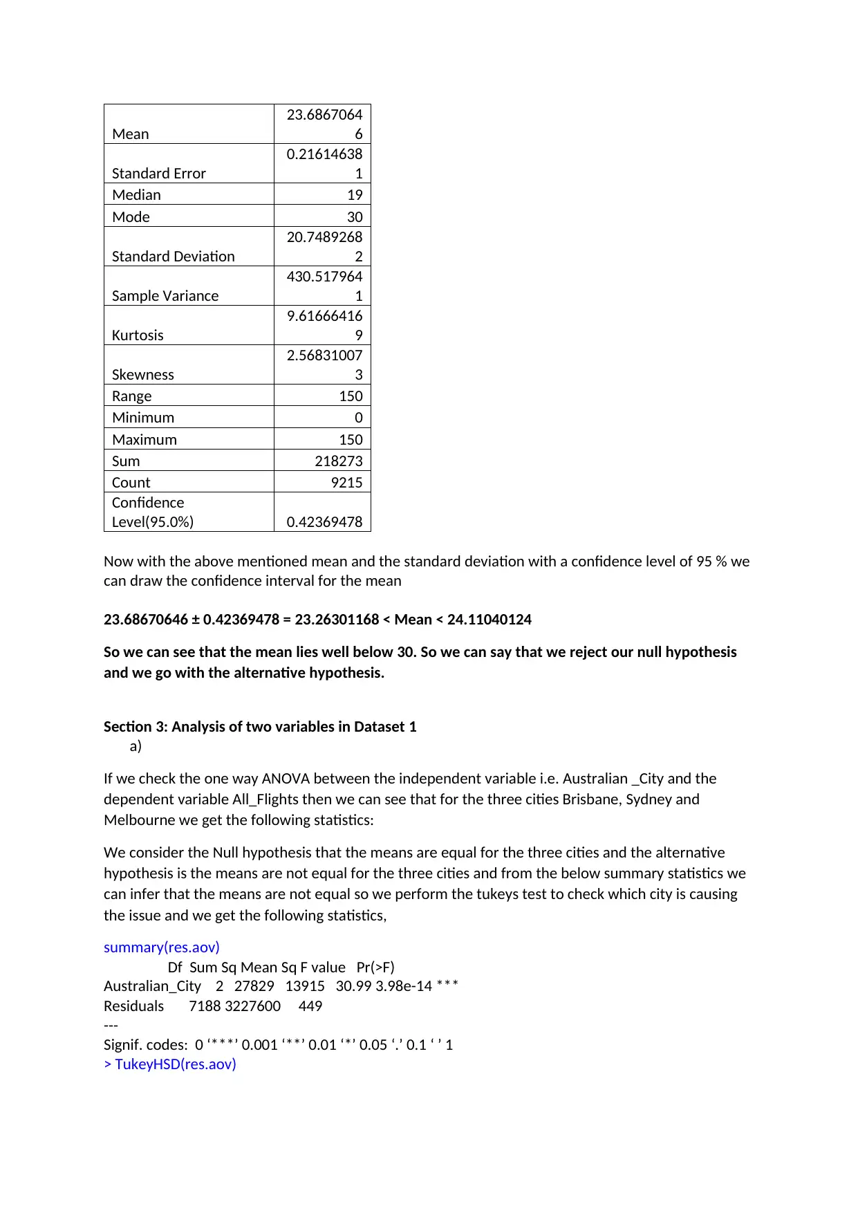
Now with the above mentioned mean and the standard deviation with a confidence level of 95 % we
can draw the confidence interval for the mean
23.68670646 ± 0.42369478 = 23.26301168 < Mean < 24.11040124
So we can see that the mean lies well below 30. So we can say that we reject our null hypothesis
and we go with the alternative hypothesis.
Section 3: Analysis of two variables in Dataset 1
a)
If we check the one way ANOVA between the independent variable i.e. Australian _City and the
dependent variable All_Flights then we can see that for the three cities Brisbane, Sydney and
Melbourne we get the following statistics:
We consider the Null hypothesis that the means are equal for the three cities and the alternative
hypothesis is the means are not equal for the three cities and from the below summary statistics we
can infer that the means are not equal so we perform the tukeys test to check which city is causing
the issue and we get the following statistics,
summary(res.aov)
Df Sum Sq Mean Sq F value Pr(>F)
Australian_City 2 27829 13915 30.99 3.98e-14 ***
Residuals 7188 3227600 449
---
Signif. codes: 0 ‘***’ 0.001 ‘**’ 0.01 ‘*’ 0.05 ‘.’ 0.1 ‘ ’ 1
> TukeyHSD(res.aov)
23.6867064
6
Standard Error
0.21614638
1
Median 19
Mode 30
Standard Deviation
20.7489268
2
Sample Variance
430.517964
1
Kurtosis
9.61666416
9
Skewness
2.56831007
3
Range 150
Minimum 0
Maximum 150
Sum 218273
Count 9215
Confidence
Level(95.0%) 0.42369478
Now with the above mentioned mean and the standard deviation with a confidence level of 95 % we
can draw the confidence interval for the mean
23.68670646 ± 0.42369478 = 23.26301168 < Mean < 24.11040124
So we can see that the mean lies well below 30. So we can say that we reject our null hypothesis
and we go with the alternative hypothesis.
Section 3: Analysis of two variables in Dataset 1
a)
If we check the one way ANOVA between the independent variable i.e. Australian _City and the
dependent variable All_Flights then we can see that for the three cities Brisbane, Sydney and
Melbourne we get the following statistics:
We consider the Null hypothesis that the means are equal for the three cities and the alternative
hypothesis is the means are not equal for the three cities and from the below summary statistics we
can infer that the means are not equal so we perform the tukeys test to check which city is causing
the issue and we get the following statistics,
summary(res.aov)
Df Sum Sq Mean Sq F value Pr(>F)
Australian_City 2 27829 13915 30.99 3.98e-14 ***
Residuals 7188 3227600 449
---
Signif. codes: 0 ‘***’ 0.001 ‘**’ 0.01 ‘*’ 0.05 ‘.’ 0.1 ‘ ’ 1
> TukeyHSD(res.aov)
Tukey multiple comparisons of means
95% family-wise confidence level
Fit: aov(formula = All_Flights ~ Australian_City, data = flightdata)
$`Australian_City`
diff lwr upr p adj
Melbourne-Brisbane 3.9015875 2.2666967 5.536478 0.0000001
Sydney-Brisbane 4.8182714 3.3654116 6.271131 0.0000000
Sydney-Melbourne 0.9166839 -0.4891996 2.322567 0.2775764
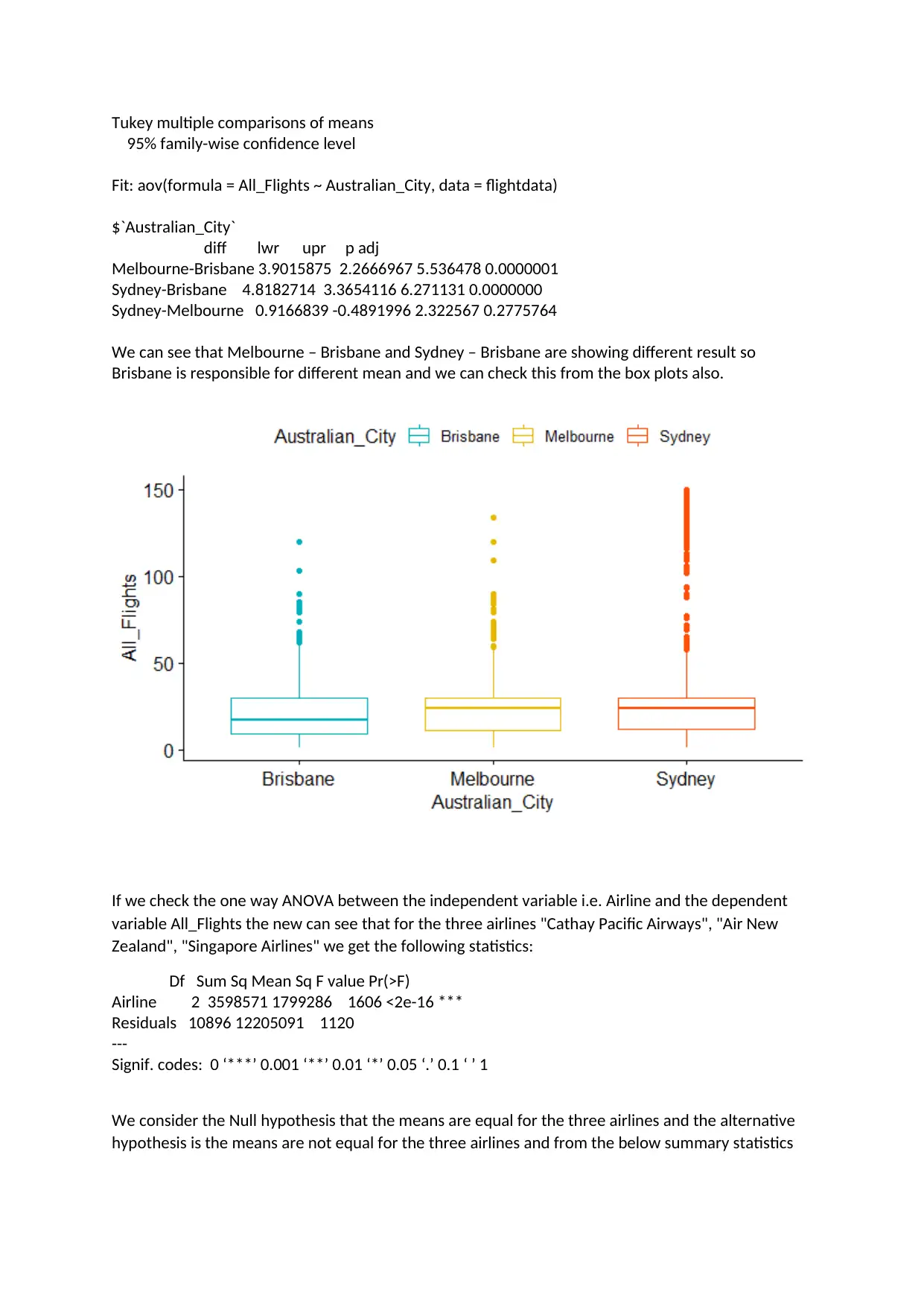
We can see that Melbourne – Brisbane and Sydney – Brisbane are showing different result so
Brisbane is responsible for different mean and we can check this from the box plots also.
If we check the one way ANOVA between the independent variable i.e. Airline and the dependent
variable All_Flights the new can see that for the three airlines "Cathay Pacific Airways", "Air New
Zealand", "Singapore Airlines" we get the following statistics:
Df Sum Sq Mean Sq F value Pr(>F)
Airline 2 3598571 1799286 1606 <2e-16 ***
Residuals 10896 12205091 1120
---
Signif. codes: 0 ‘***’ 0.001 ‘**’ 0.01 ‘*’ 0.05 ‘.’ 0.1 ‘ ’ 1
We consider the Null hypothesis that the means are equal for the three airlines and the alternative
hypothesis is the means are not equal for the three airlines and from the below summary statistics
95% family-wise confidence level
Fit: aov(formula = All_Flights ~ Australian_City, data = flightdata)
$`Australian_City`
diff lwr upr p adj
Melbourne-Brisbane 3.9015875 2.2666967 5.536478 0.0000001
Sydney-Brisbane 4.8182714 3.3654116 6.271131 0.0000000
Sydney-Melbourne 0.9166839 -0.4891996 2.322567 0.2775764
We can see that Melbourne – Brisbane and Sydney – Brisbane are showing different result so
Brisbane is responsible for different mean and we can check this from the box plots also.
If we check the one way ANOVA between the independent variable i.e. Airline and the dependent
variable All_Flights the new can see that for the three airlines "Cathay Pacific Airways", "Air New
Zealand", "Singapore Airlines" we get the following statistics:
Df Sum Sq Mean Sq F value Pr(>F)
Airline 2 3598571 1799286 1606 <2e-16 ***
Residuals 10896 12205091 1120
---
Signif. codes: 0 ‘***’ 0.001 ‘**’ 0.01 ‘*’ 0.05 ‘.’ 0.1 ‘ ’ 1
We consider the Null hypothesis that the means are equal for the three airlines and the alternative
hypothesis is the means are not equal for the three airlines and from the below summary statistics
⊘ This is a preview!⊘
Do you want full access?
Subscribe today to unlock all pages.
Trusted by 1+ million students worldwide
we can infer that the means are not equal so we perform the tukeys test to check which city is
causing the issue and we get the following statistics,
Tukey multiple comparisons of means
95% family-wise confidence level
Fit: aov(formula = All_Flights ~ Airline, data = flightdata)
$`Airline`
diff lwr upr p adj
Cathay Pacific Airways-Air New Zealand 1.689022 -0.0636793 3.441723 0.0617867
Singapore Airlines-Air New Zealand 49.711294 47.5980450 51.824544 0.0000000
Singapore Airlines-Cathay Pacific Airways 48.022272 45.6691995 50.375345 0.0000000
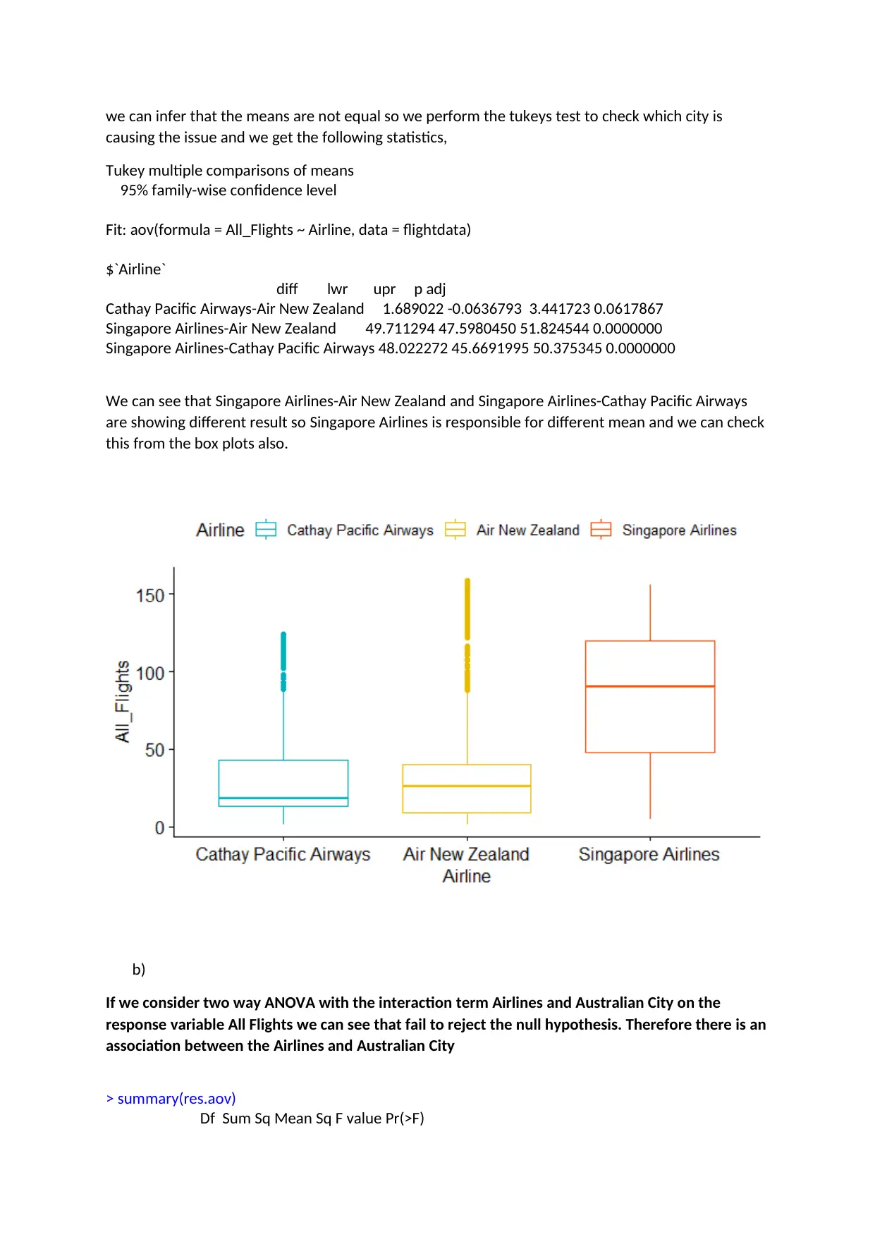
We can see that Singapore Airlines-Air New Zealand and Singapore Airlines-Cathay Pacific Airways
are showing different result so Singapore Airlines is responsible for different mean and we can check
this from the box plots also.
b)
If we consider two way ANOVA with the interaction term Airlines and Australian City on the
response variable All Flights we can see that fail to reject the null hypothesis. Therefore there is an
association between the Airlines and Australian City
> summary(res.aov)
Df Sum Sq Mean Sq F value Pr(>F)
causing the issue and we get the following statistics,
Tukey multiple comparisons of means
95% family-wise confidence level
Fit: aov(formula = All_Flights ~ Airline, data = flightdata)
$`Airline`
diff lwr upr p adj
Cathay Pacific Airways-Air New Zealand 1.689022 -0.0636793 3.441723 0.0617867
Singapore Airlines-Air New Zealand 49.711294 47.5980450 51.824544 0.0000000
Singapore Airlines-Cathay Pacific Airways 48.022272 45.6691995 50.375345 0.0000000
We can see that Singapore Airlines-Air New Zealand and Singapore Airlines-Cathay Pacific Airways
are showing different result so Singapore Airlines is responsible for different mean and we can check
this from the box plots also.
b)
If we consider two way ANOVA with the interaction term Airlines and Australian City on the
response variable All Flights we can see that fail to reject the null hypothesis. Therefore there is an
association between the Airlines and Australian City
> summary(res.aov)
Df Sum Sq Mean Sq F value Pr(>F)
Paraphrase This Document
Need a fresh take? Get an instant paraphrase of this document with our AI Paraphraser
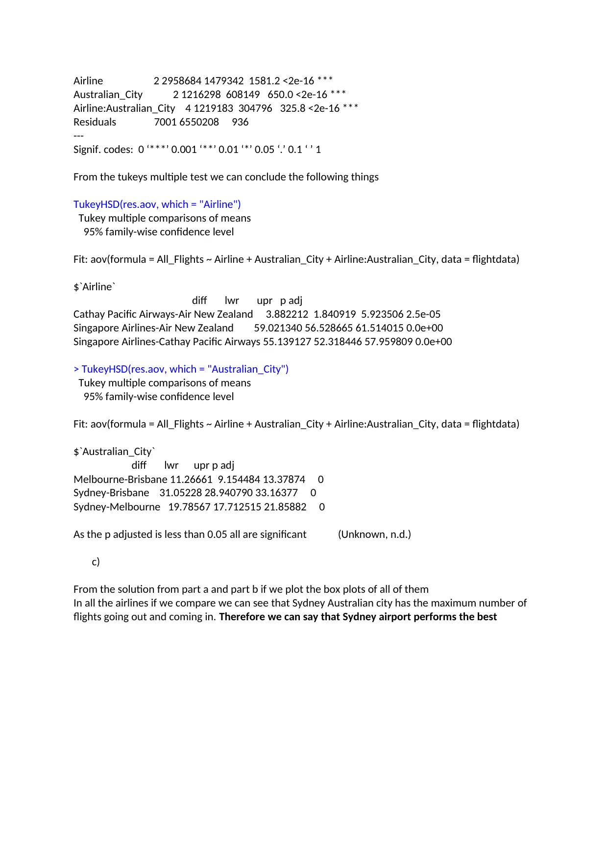
Airline 2 2958684 1479342 1581.2 <2e-16 ***
Australian_City 2 1216298 608149 650.0 <2e-16 ***
Airline:Australian_City 4 1219183 304796 325.8 <2e-16 ***
Residuals 7001 6550208 936
---
Signif. codes: 0 ‘***’ 0.001 ‘**’ 0.01 ‘*’ 0.05 ‘.’ 0.1 ‘ ’ 1
From the tukeys multiple test we can conclude the following things
TukeyHSD(res.aov, which = "Airline")
Tukey multiple comparisons of means
95% family-wise confidence level
Fit: aov(formula = All_Flights ~ Airline + Australian_City + Airline:Australian_City, data = flightdata)
$`Airline`
diff lwr upr p adj
Cathay Pacific Airways-Air New Zealand 3.882212 1.840919 5.923506 2.5e-05
Singapore Airlines-Air New Zealand 59.021340 56.528665 61.514015 0.0e+00
Singapore Airlines-Cathay Pacific Airways 55.139127 52.318446 57.959809 0.0e+00
> TukeyHSD(res.aov, which = "Australian_City")
Tukey multiple comparisons of means
95% family-wise confidence level
Fit: aov(formula = All_Flights ~ Airline + Australian_City + Airline:Australian_City, data = flightdata)
$`Australian_City`
diff lwr upr p adj
Melbourne-Brisbane 11.26661 9.154484 13.37874 0
Sydney-Brisbane 31.05228 28.940790 33.16377 0
Sydney-Melbourne 19.78567 17.712515 21.85882 0
As the p adjusted is less than 0.05 all are significant (Unknown, n.d.)
c)
From the solution from part a and part b if we plot the box plots of all of them
In all the airlines if we compare we can see that Sydney Australian city has the maximum number of
flights going out and coming in. Therefore we can say that Sydney airport performs the best
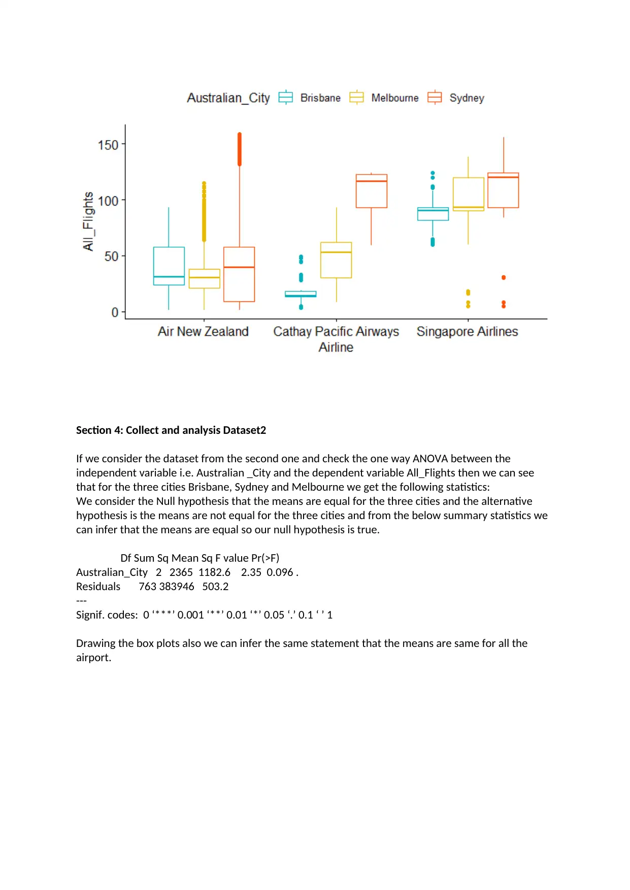
Section 4: Collect and analysis Dataset2
If we consider the dataset from the second one and check the one way ANOVA between the
independent variable i.e. Australian _City and the dependent variable All_Flights then we can see
that for the three cities Brisbane, Sydney and Melbourne we get the following statistics:
We consider the Null hypothesis that the means are equal for the three cities and the alternative
hypothesis is the means are not equal for the three cities and from the below summary statistics we
can infer that the means are equal so our null hypothesis is true.
Df Sum Sq Mean Sq F value Pr(>F)
Australian_City 2 2365 1182.6 2.35 0.096 .
Residuals 763 383946 503.2
---
Signif. codes: 0 ‘***’ 0.001 ‘**’ 0.01 ‘*’ 0.05 ‘.’ 0.1 ‘ ’ 1
Drawing the box plots also we can infer the same statement that the means are same for all the
airport.
⊘ This is a preview!⊘
Do you want full access?
Subscribe today to unlock all pages.
Trusted by 1+ million students worldwide
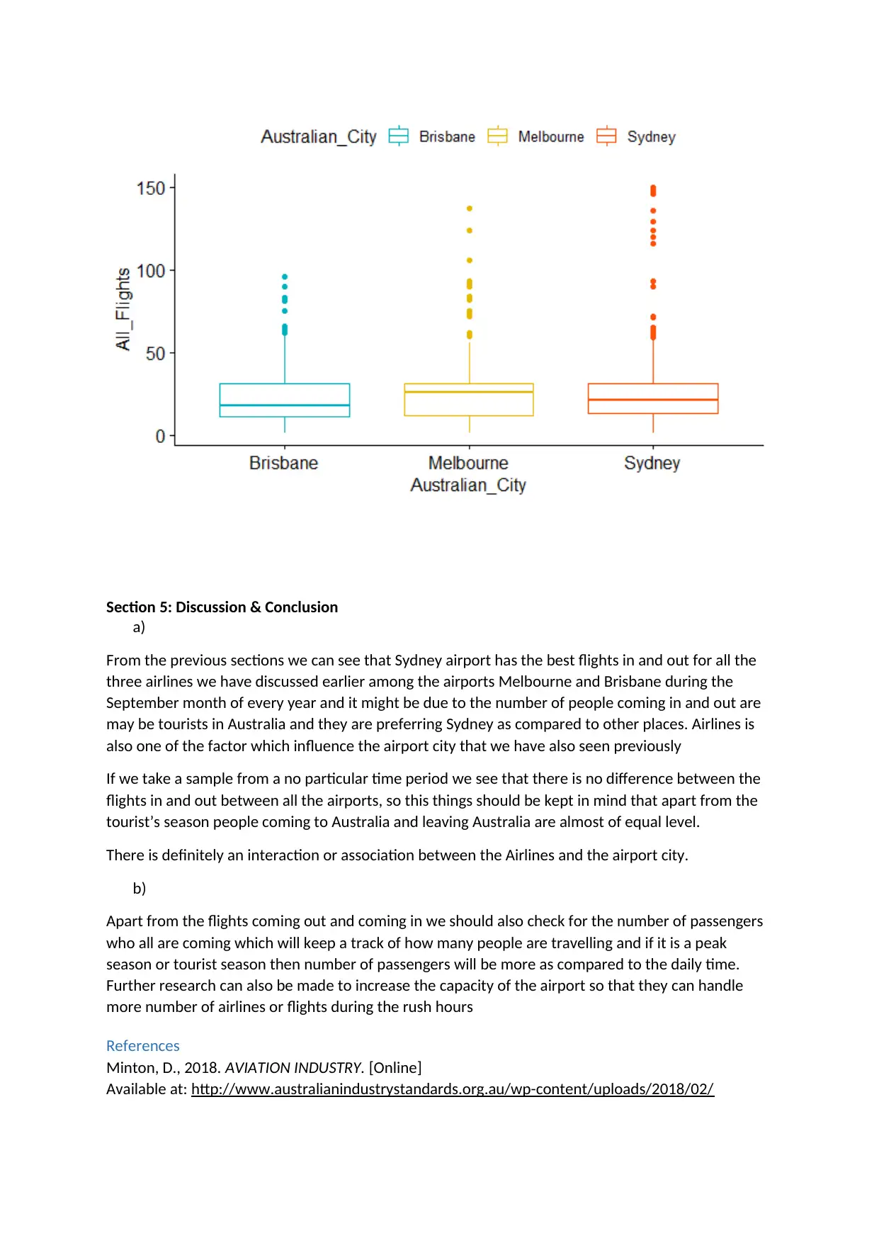
Section 5: Discussion & Conclusion
a)
From the previous sections we can see that Sydney airport has the best flights in and out for all the
three airlines we have discussed earlier among the airports Melbourne and Brisbane during the
September month of every year and it might be due to the number of people coming in and out are
may be tourists in Australia and they are preferring Sydney as compared to other places. Airlines is
also one of the factor which influence the airport city that we have also seen previously
If we take a sample from a no particular time period we see that there is no difference between the
flights in and out between all the airports, so this things should be kept in mind that apart from the
tourist’s season people coming to Australia and leaving Australia are almost of equal level.
There is definitely an interaction or association between the Airlines and the airport city.
b)
Apart from the flights coming out and coming in we should also check for the number of passengers
who all are coming which will keep a track of how many people are travelling and if it is a peak
season or tourist season then number of passengers will be more as compared to the daily time.
Further research can also be made to increase the capacity of the airport so that they can handle
more number of airlines or flights during the rush hours
References
Minton, D., 2018. AVIATION INDUSTRY. [Online]
Available at: http://www.australianindustrystandards.org.au/wp-content/uploads/2018/02/
Paraphrase This Document
Need a fresh take? Get an instant paraphrase of this document with our AI Paraphraser

Aviation-Key-Findings-Paper2018V4Web.pdf
[Accessed 27 Jan 2019].
Unknown, n.d. Statistical tools for high-throughput data analysis. [Online]
Available at: http://www.sthda.com/english/wiki/two-way-anova-test-in-r
[Accessed 27 Jan 2019].
[Accessed 27 Jan 2019].
Unknown, n.d. Statistical tools for high-throughput data analysis. [Online]
Available at: http://www.sthda.com/english/wiki/two-way-anova-test-in-r
[Accessed 27 Jan 2019].
1 out of 11
Related Documents


Your All-in-One AI-Powered Toolkit for Academic Success.
+13062052269
info@desklib.com
Available 24*7 on WhatsApp / Email
![[object Object]](/_next/static/media/star-bottom.7253800d.svg)
Unlock your academic potential
Copyright © 2020–2026 A2Z Services. All Rights Reserved. Developed and managed by ZUCOL.