MGT2320 Assignment 3: Case Study, ABC Analysis, and EOQ Solutions
VerifiedAdded on 2022/11/19
|11
|2300
|168
Homework Assignment
AI Summary
This document presents a comprehensive solution to MGT2320 Assignment 3, focusing on layout design, inventory management, and Economic Order Quantity (EOQ) calculations. The assignment begins with a case study analyzing the layout of a manufacturing facility, evaluating the movement cost of the current layout and proposing a new layout to reduce costs. It then delves into inventory management, utilizing ABC analysis to classify items based on their value and applying cycle counting techniques for efficient inventory control. Finally, the solution addresses EOQ, calculating the optimal order quantity, average inventory levels, annual holding costs, number of orders, and annual ordering costs. The document provides detailed calculations, tables, and figures to support the analysis, offering valuable insights into operations management principles.
MGT2320 – Assignment 3
ALGONQUIN COLLEGE
Centre for Continuing & Online Learning
Course Name
Name of Student
Submission Date
ALGONQUIN COLLEGE
Centre for Continuing & Online Learning
Course Name
Name of Student
Submission Date
Paraphrase This Document
Need a fresh take? Get an instant paraphrase of this document with our AI Paraphraser
Table of Contents
Table of Contents.......................................................................................................................2
1. Case Study – Types of Layout...............................................................................................3
2. Load and Movement Cost......................................................................................................6
2.A The movement cost of the current layout........................................................................6
2.B New layout with lower movement cost...........................................................................6
3 ABC Analysis..........................................................................................................................8
3.A Classification of items by ABC analysis.........................................................................8
3.B Application of ABC analysis...........................................................................................8
4. Cycle Counting.......................................................................................................................9
5. EOQ........................................................................................................................................9
List of Tables
Table 1: New Layout after re-arranging the stations according to the movement.....................7
Table 2: Inventory classification criteria for ABC analysis.......................................................8
Table 3: Cycle counting calculation for per day count..............................................................9
List of Figures
Figure 1: Layout of the new location.........................................................................................3
Figure 2: ABC analysis for classification of items....................................................................8
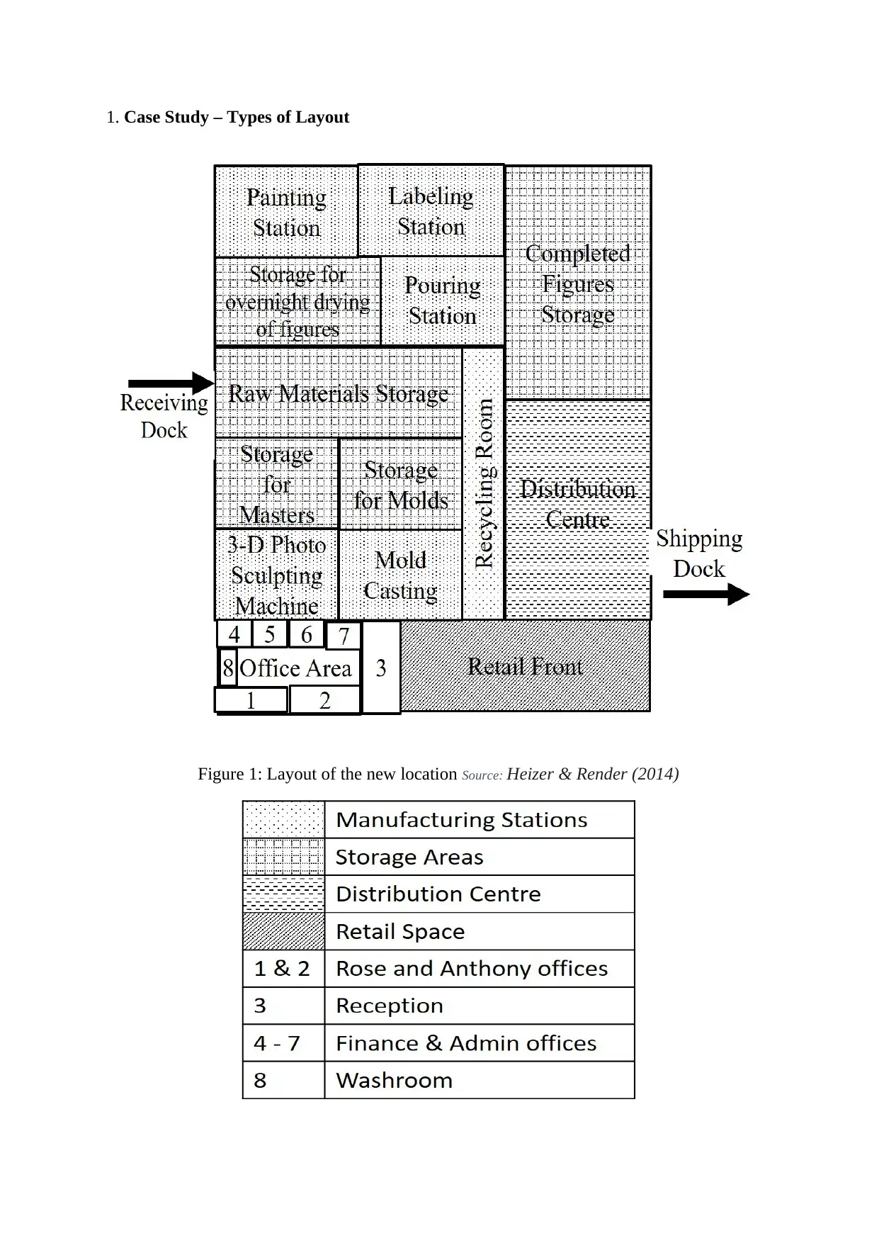
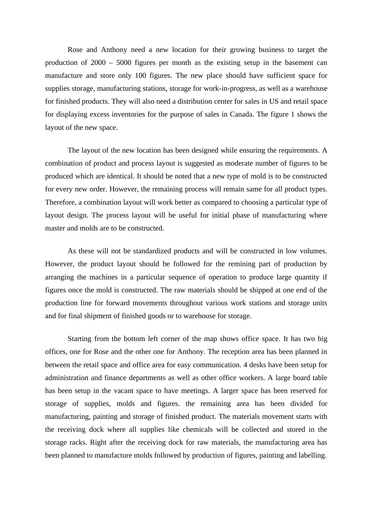
1. Case Study – Types of Layout
Figure 1: Layout of the new location Source: Heizer & Render (2014)
Figure 1: Layout of the new location Source: Heizer & Render (2014)
⊘ This is a preview!⊘
Do you want full access?
Subscribe today to unlock all pages.
Trusted by 1+ million students worldwide
Rose and Anthony need a new location for their growing business to target the
production of 2000 – 5000 figures per month as the existing setup in the basement can
manufacture and store only 100 figures. The new place should have sufficient space for
supplies storage, manufacturing stations, storage for work-in-progress, as well as a warehouse
for finished products. They will also need a distribution center for sales in US and retail space
for displaying excess inventories for the purpose of sales in Canada. The figure 1 shows the
layout of the new space.
The layout of the new location has been designed while ensuring the requirements. A
combination of product and process layout is suggested as moderate number of figures to be
produced which are identical. It should be noted that a new type of mold is to be constructed
for every new order. However, the remaining process will remain same for all product types.
Therefore, a combination layout will work better as compared to choosing a particular type of
layout design. The process layout will be useful for initial phase of manufacturing where
master and molds are to be constructed.
As these will not be standardized products and will be constructed in low volumes.
However, the product layout should be followed for the remining part of production by
arranging the machines in a particular sequence of operation to produce large quantity if
figures once the mold is constructed. The raw materials should be shipped at one end of the
production line for forward movements throughout various work stations and storage units
and for final shipment of finished goods or to warehouse for storage.
Starting from the bottom left corner of the map shows office space. It has two big
offices, one for Rose and the other one for Anthony. The reception area has been planned in
between the retail space and office area for easy communication. 4 desks have been setup for
administration and finance departments as well as other office workers. A large board table
has been setup in the vacant space to have meetings. A larger space has been reserved for
storage of supplies, molds and figures. the remaining area has been divided for
manufacturing, painting and storage of finished product. The materials movement starts with
the receiving dock where all supplies like chemicals will be collected and stored in the
storage racks. Right after the receiving dock for raw materials, the manufacturing area has
been planned to manufacture molds followed by production of figures, painting and labelling.
Paraphrase This Document
Need a fresh take? Get an instant paraphrase of this document with our AI Paraphraser
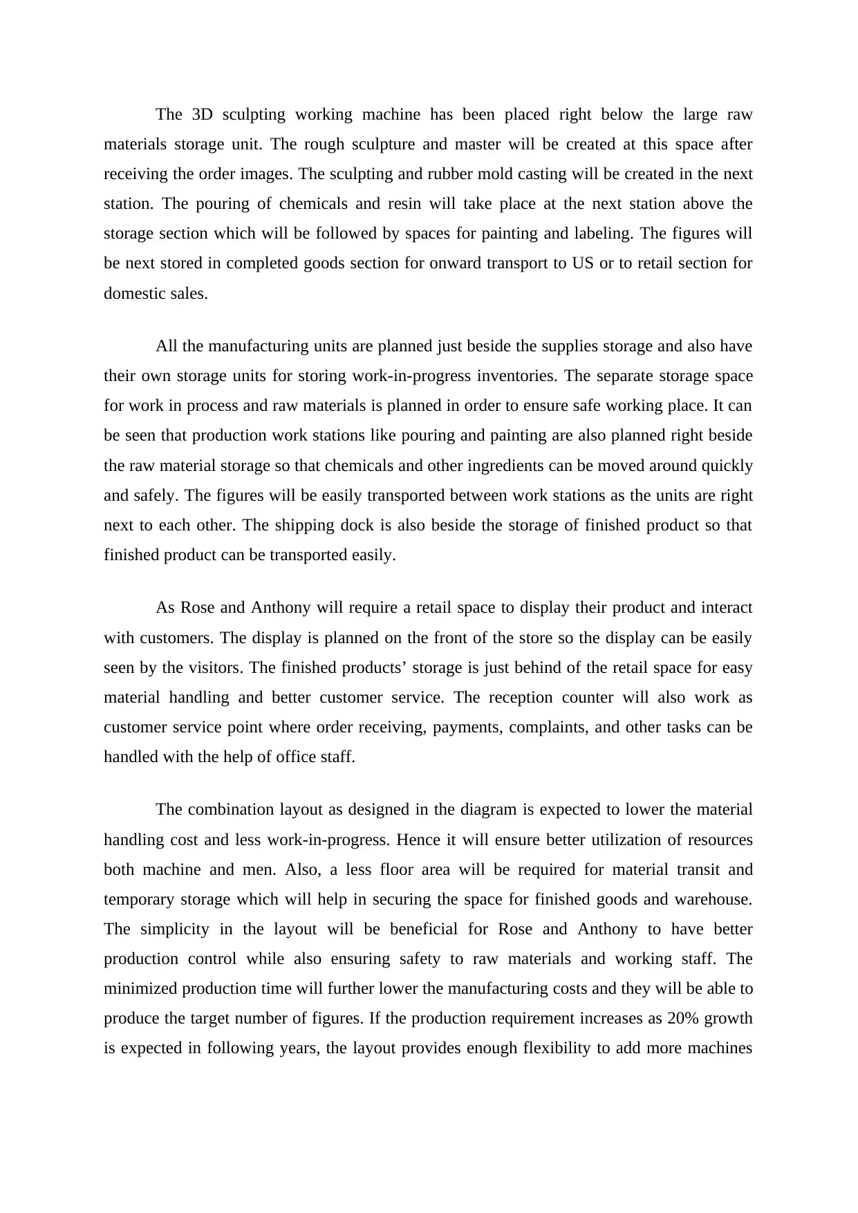
The 3D sculpting working machine has been placed right below the large raw
materials storage unit. The rough sculpture and master will be created at this space after
receiving the order images. The sculpting and rubber mold casting will be created in the next
station. The pouring of chemicals and resin will take place at the next station above the
storage section which will be followed by spaces for painting and labeling. The figures will
be next stored in completed goods section for onward transport to US or to retail section for
domestic sales.
All the manufacturing units are planned just beside the supplies storage and also have
their own storage units for storing work-in-progress inventories. The separate storage space
for work in process and raw materials is planned in order to ensure safe working place. It can
be seen that production work stations like pouring and painting are also planned right beside
the raw material storage so that chemicals and other ingredients can be moved around quickly
and safely. The figures will be easily transported between work stations as the units are right
next to each other. The shipping dock is also beside the storage of finished product so that
finished product can be transported easily.
As Rose and Anthony will require a retail space to display their product and interact
with customers. The display is planned on the front of the store so the display can be easily
seen by the visitors. The finished products’ storage is just behind of the retail space for easy
material handling and better customer service. The reception counter will also work as
customer service point where order receiving, payments, complaints, and other tasks can be
handled with the help of office staff.
The combination layout as designed in the diagram is expected to lower the material
handling cost and less work-in-progress. Hence it will ensure better utilization of resources
both machine and men. Also, a less floor area will be required for material transit and
temporary storage which will help in securing the space for finished goods and warehouse.
The simplicity in the layout will be beneficial for Rose and Anthony to have better
production control while also ensuring safety to raw materials and working staff. The
minimized production time will further lower the manufacturing costs and they will be able to
produce the target number of figures. If the production requirement increases as 20% growth
is expected in following years, the layout provides enough flexibility to add more machines
in respective work stations along with enough temporary space to accommodate the work in
process.
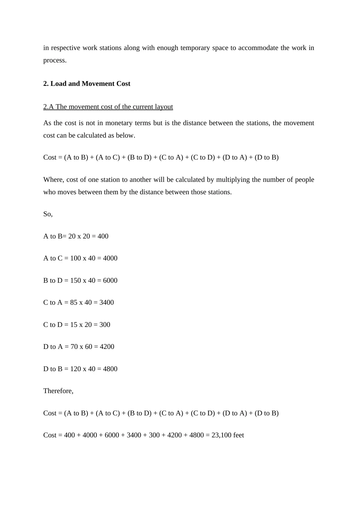
2. Load and Movement Cost
2.A The movement cost of the current layout
As the cost is not in monetary terms but is the distance between the stations, the movement
cost can be calculated as below.
Cost = (A to B) + (A to C) + (B to D) + (C to A) + (C to D) + (D to A) + (D to B)
Where, cost of one station to another will be calculated by multiplying the number of people
who moves between them by the distance between those stations.
So,
A to B= 20 x 20 = 400
A to C = 100 x 40 = 4000
B to D = 150 x 40 = 6000
C to A = 85 x 40 = 3400
C to D = 15 x 20 = 300
D to A = 70 x 60 = 4200
D to B = 120 x 40 = 4800
Therefore,
Cost = (A to B) + (A to C) + (B to D) + (C to A) + (C to D) + (D to A) + (D to B)
Cost = 400 + 4000 + 6000 + 3400 + 300 + 4200 + 4800 = 23,100 feet
process.
2. Load and Movement Cost
2.A The movement cost of the current layout
As the cost is not in monetary terms but is the distance between the stations, the movement
cost can be calculated as below.
Cost = (A to B) + (A to C) + (B to D) + (C to A) + (C to D) + (D to A) + (D to B)
Where, cost of one station to another will be calculated by multiplying the number of people
who moves between them by the distance between those stations.
So,
A to B= 20 x 20 = 400
A to C = 100 x 40 = 4000
B to D = 150 x 40 = 6000
C to A = 85 x 40 = 3400
C to D = 15 x 20 = 300
D to A = 70 x 60 = 4200
D to B = 120 x 40 = 4800
Therefore,
Cost = (A to B) + (A to C) + (B to D) + (C to A) + (C to D) + (D to A) + (D to B)
Cost = 400 + 4000 + 6000 + 3400 + 300 + 4200 + 4800 = 23,100 feet
⊘ This is a preview!⊘
Do you want full access?
Subscribe today to unlock all pages.
Trusted by 1+ million students worldwide
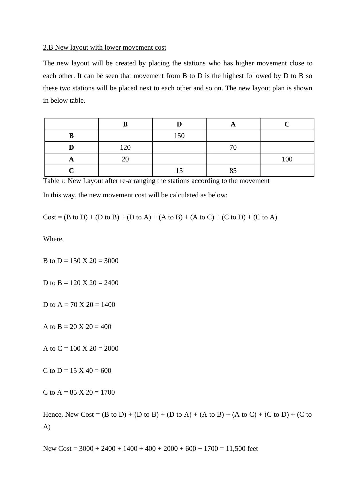
2.B New layout with lower movement cost
The new layout will be created by placing the stations who has higher movement close to
each other. It can be seen that movement from B to D is the highest followed by D to B so
these two stations will be placed next to each other and so on. The new layout plan is shown
in below table.
B D A C
B 150
D 120 70
A 20 100
C 15 85
Table 1: New Layout after re-arranging the stations according to the movement
In this way, the new movement cost will be calculated as below:
Cost = (B to D) + (D to B) + (D to A) + (A to B) + (A to C) + (C to D) + (C to A)
Where,
B to D = 150 X 20 = 3000
D to B = 120 X 20 = 2400
D to A = 70 X 20 = 1400
A to B = 20 X 20 = 400
A to C = 100 X 20 = 2000
C to D = 15 X 40 = 600
C to A = 85 X 20 = 1700
Hence, New Cost = (B to D) + (D to B) + (D to A) + (A to B) + (A to C) + (C to D) + (C to
A)
New Cost = 3000 + 2400 + 1400 + 400 + 2000 + 600 + 1700 = 11,500 feet
Paraphrase This Document
Need a fresh take? Get an instant paraphrase of this document with our AI Paraphraser
Therefore, the movement cost saving is =
Old cost – New cost = 23100-11500 = 11,600 feet
3 ABC Analysis
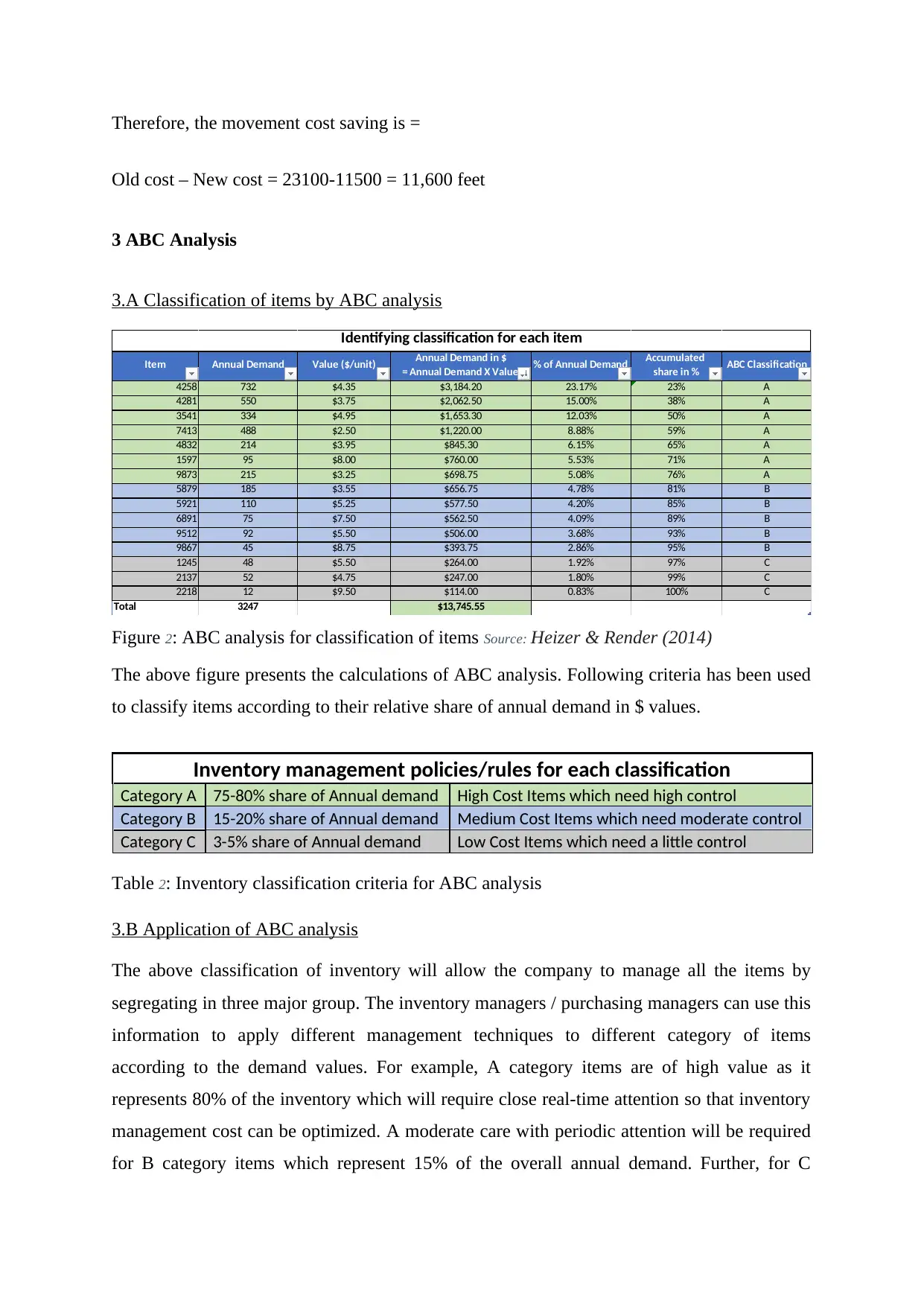
3.A Classification of items by ABC analysis
Item Annual Demand Value ($/unit) Annual Demand in $
= Annual Demand X Value % of Annual Demand Accumulated
share in % ABC Classification
4258 732 $4.35 $3,184.20 23.17% 23% A
4281 550 $3.75 $2,062.50 15.00% 38% A
3541 334 $4.95 $1,653.30 12.03% 50% A
7413 488 $2.50 $1,220.00 8.88% 59% A
4832 214 $3.95 $845.30 6.15% 65% A
1597 95 $8.00 $760.00 5.53% 71% A
9873 215 $3.25 $698.75 5.08% 76% A
5879 185 $3.55 $656.75 4.78% 81% B
5921 110 $5.25 $577.50 4.20% 85% B
6891 75 $7.50 $562.50 4.09% 89% B
9512 92 $5.50 $506.00 3.68% 93% B
9867 45 $8.75 $393.75 2.86% 95% B
1245 48 $5.50 $264.00 1.92% 97% C
2137 52 $4.75 $247.00 1.80% 99% C
2218 12 $9.50 $114.00 0.83% 100% C
Total 3247 $13,745.55
Identifying classification for each item
Figure 2: ABC analysis for classification of items Source: Heizer & Render (2014)
The above figure presents the calculations of ABC analysis. Following criteria has been used
to classify items according to their relative share of annual demand in $ values.
Inventory management policies/rules for each classification
Category A 75-80% share of Annual demand High Cost Items which need high control
Category B 15-20% share of Annual demand Medium Cost Items which need moderate control
Category C 3-5% share of Annual demand Low Cost Items which need a little control
Table 2: Inventory classification criteria for ABC analysis
3.B Application of ABC analysis
The above classification of inventory will allow the company to manage all the items by
segregating in three major group. The inventory managers / purchasing managers can use this
information to apply different management techniques to different category of items
according to the demand values. For example, A category items are of high value as it
represents 80% of the inventory which will require close real-time attention so that inventory
management cost can be optimized. A moderate care with periodic attention will be required
for B category items which represent 15% of the overall annual demand. Further, for C
Old cost – New cost = 23100-11500 = 11,600 feet
3 ABC Analysis
3.A Classification of items by ABC analysis
Item Annual Demand Value ($/unit) Annual Demand in $
= Annual Demand X Value % of Annual Demand Accumulated
share in % ABC Classification
4258 732 $4.35 $3,184.20 23.17% 23% A
4281 550 $3.75 $2,062.50 15.00% 38% A
3541 334 $4.95 $1,653.30 12.03% 50% A
7413 488 $2.50 $1,220.00 8.88% 59% A
4832 214 $3.95 $845.30 6.15% 65% A
1597 95 $8.00 $760.00 5.53% 71% A
9873 215 $3.25 $698.75 5.08% 76% A
5879 185 $3.55 $656.75 4.78% 81% B
5921 110 $5.25 $577.50 4.20% 85% B
6891 75 $7.50 $562.50 4.09% 89% B
9512 92 $5.50 $506.00 3.68% 93% B
9867 45 $8.75 $393.75 2.86% 95% B
1245 48 $5.50 $264.00 1.92% 97% C
2137 52 $4.75 $247.00 1.80% 99% C
2218 12 $9.50 $114.00 0.83% 100% C
Total 3247 $13,745.55
Identifying classification for each item
Figure 2: ABC analysis for classification of items Source: Heizer & Render (2014)
The above figure presents the calculations of ABC analysis. Following criteria has been used
to classify items according to their relative share of annual demand in $ values.
Inventory management policies/rules for each classification
Category A 75-80% share of Annual demand High Cost Items which need high control
Category B 15-20% share of Annual demand Medium Cost Items which need moderate control
Category C 3-5% share of Annual demand Low Cost Items which need a little control
Table 2: Inventory classification criteria for ABC analysis
3.B Application of ABC analysis
The above classification of inventory will allow the company to manage all the items by
segregating in three major group. The inventory managers / purchasing managers can use this
information to apply different management techniques to different category of items
according to the demand values. For example, A category items are of high value as it
represents 80% of the inventory which will require close real-time attention so that inventory
management cost can be optimized. A moderate care with periodic attention will be required
for B category items which represent 15% of the overall annual demand. Further, for C
category items relaxed inventory processes can be employed as it represents only 5% of the
annual demand value. In this way, the strategic cost management technique will help the
management to increase revenue and decrease costs by optimum utilization of resources.
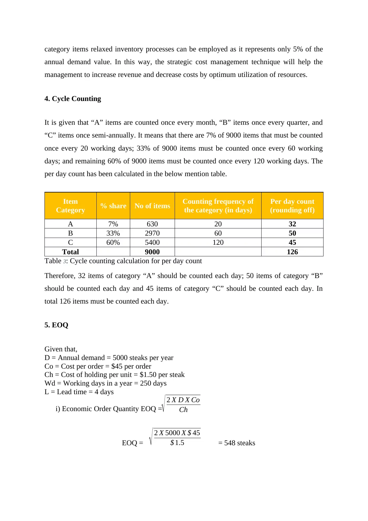
4. Cycle Counting
It is given that “A” items are counted once every month, “B” items once every quarter, and
“C” items once semi-annually. It means that there are 7% of 9000 items that must be counted
once every 20 working days; 33% of 9000 items must be counted once every 60 working
days; and remaining 60% of 9000 items must be counted once every 120 working days. The
per day count has been calculated in the below mention table.
Item
Category % share No of items Counting frequency of
the category (in days)
Per day count
(rounding off)
A 7% 630 20 32
B 33% 2970 60 50
C 60% 5400 120 45
Total 9000 126
Table 3: Cycle counting calculation for per day count
Therefore, 32 items of category “A” should be counted each day; 50 items of category “B”
should be counted each day and 45 items of category “C” should be counted each day. In
total 126 items must be counted each day.
5. EOQ
Given that,
D = Annual demand = 5000 steaks per year
Co = Cost per order = $45 per order
Ch = Cost of holding per unit = $1.50 per steak
Wd = Working days in a year = 250 days
L = Lead time = 4 days
i) Economic Order Quantity EOQ =
EOQ = = 548 steaks
√ 2 X D X Co
Ch
√ 2 X 5000 X $ 45
$ 1.5
annual demand value. In this way, the strategic cost management technique will help the
management to increase revenue and decrease costs by optimum utilization of resources.
4. Cycle Counting
It is given that “A” items are counted once every month, “B” items once every quarter, and
“C” items once semi-annually. It means that there are 7% of 9000 items that must be counted
once every 20 working days; 33% of 9000 items must be counted once every 60 working
days; and remaining 60% of 9000 items must be counted once every 120 working days. The
per day count has been calculated in the below mention table.
Item
Category % share No of items Counting frequency of
the category (in days)
Per day count
(rounding off)
A 7% 630 20 32
B 33% 2970 60 50
C 60% 5400 120 45
Total 9000 126
Table 3: Cycle counting calculation for per day count
Therefore, 32 items of category “A” should be counted each day; 50 items of category “B”
should be counted each day and 45 items of category “C” should be counted each day. In
total 126 items must be counted each day.
5. EOQ
Given that,
D = Annual demand = 5000 steaks per year
Co = Cost per order = $45 per order
Ch = Cost of holding per unit = $1.50 per steak
Wd = Working days in a year = 250 days
L = Lead time = 4 days
i) Economic Order Quantity EOQ =
EOQ = = 548 steaks
√ 2 X D X Co
Ch
√ 2 X 5000 X $ 45
$ 1.5
⊘ This is a preview!⊘
Do you want full access?
Subscribe today to unlock all pages.
Trusted by 1+ million students worldwide
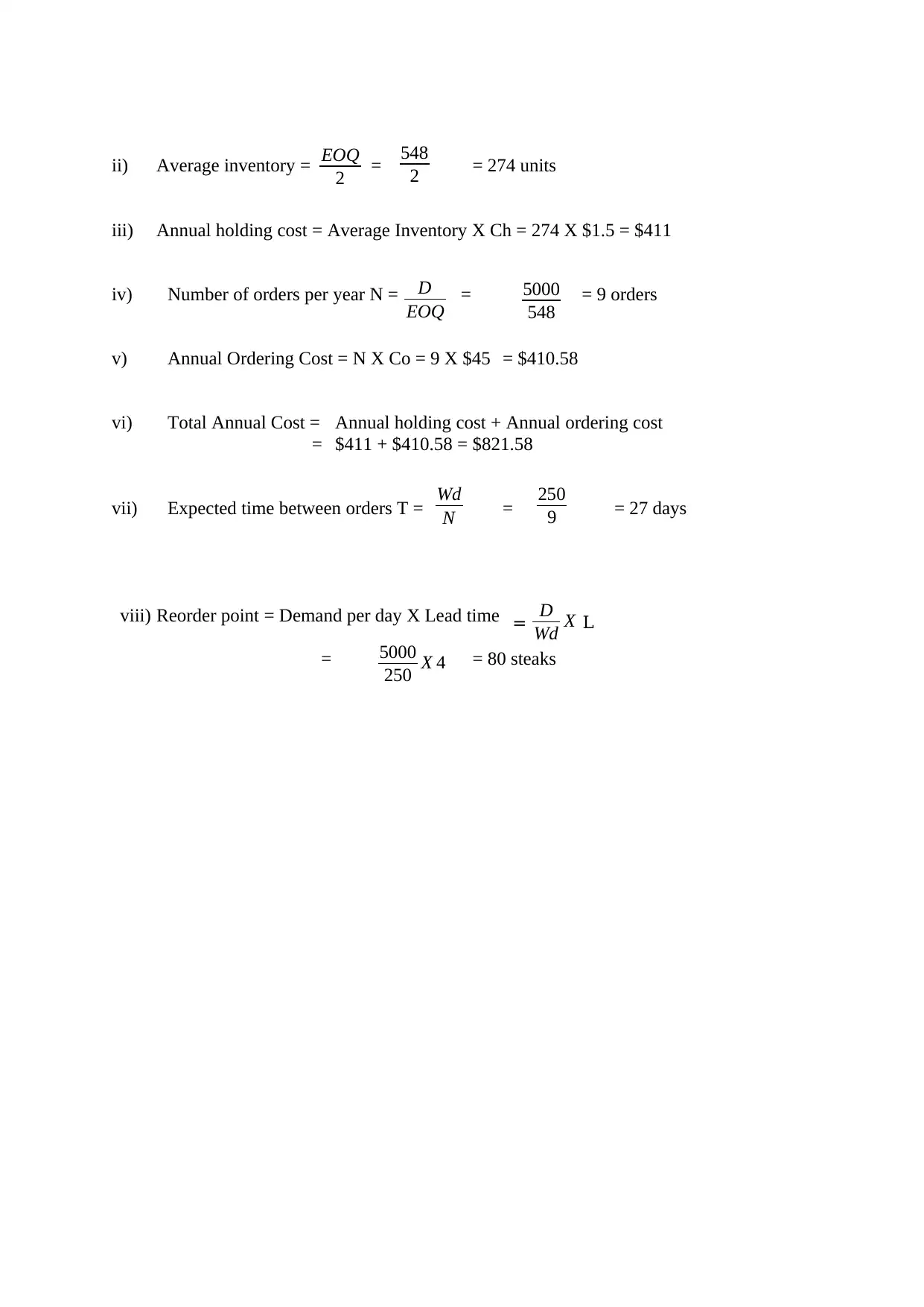
ii) Average inventory = = = 274 units
iii) Annual holding cost = Average Inventory X Ch = 274 X $1.5 = $411
iv) Number of orders per year N = = = 9 orders
v) Annual Ordering Cost = N X Co = 9 X $45 = $410.58
vi) Total Annual Cost = Annual holding cost + Annual ordering cost
= $411 + $410.58 = $821.58
vii) Expected time between orders T = = = 27 days
viii) Reorder point = Demand per day X Lead time
= = 80 steaks
EOQ
2
548
2
D
EOQ
5000
548
Wd
N
250
9
= D
Wd X L
5000
250 X 4
Paraphrase This Document
Need a fresh take? Get an instant paraphrase of this document with our AI Paraphraser
References
Heizer, J., & Render, B. (2014). Sustainability and supply chain management. Operations
Management.
Heizer, J., & Render, B. (2014). Sustainability and supply chain management. Operations
Management.
1 out of 11


Your All-in-One AI-Powered Toolkit for Academic Success.
+13062052269
info@desklib.com
Available 24*7 on WhatsApp / Email
![[object Object]](/_next/static/media/star-bottom.7253800d.svg)
Unlock your academic potential
Copyright © 2020–2026 A2Z Services. All Rights Reserved. Developed and managed by ZUCOL.