Economics 150.001 Assignment - American University Spring 2020

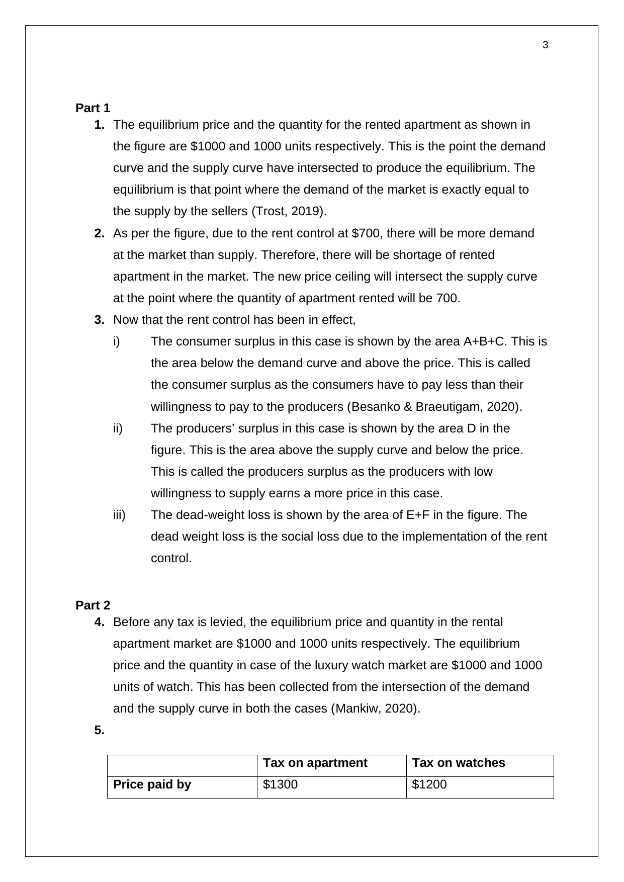
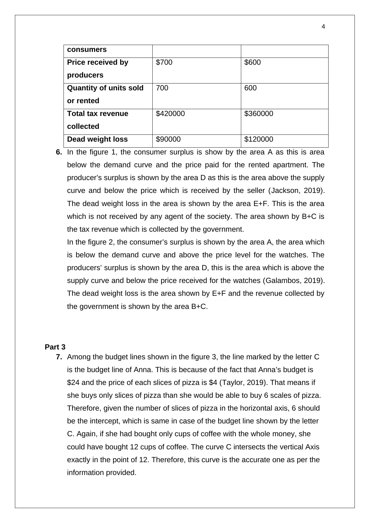
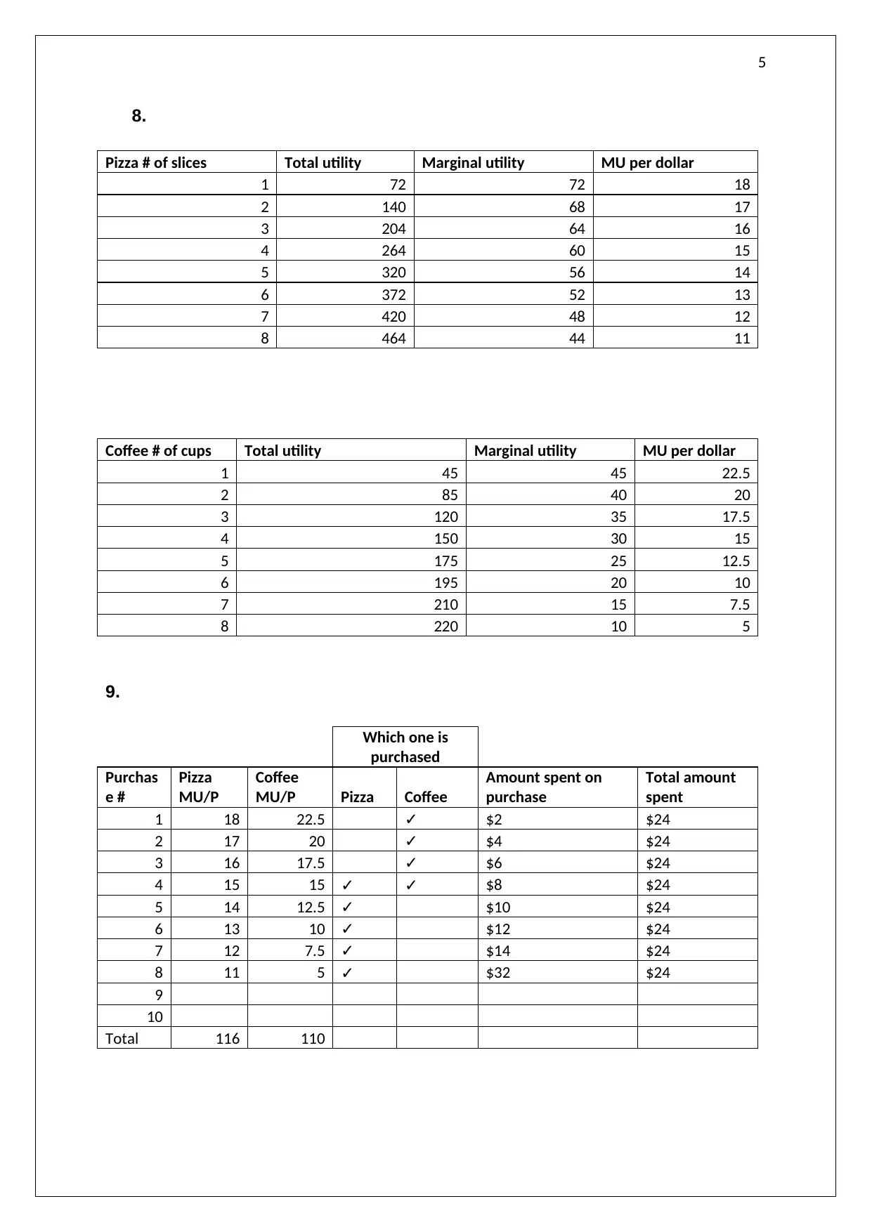
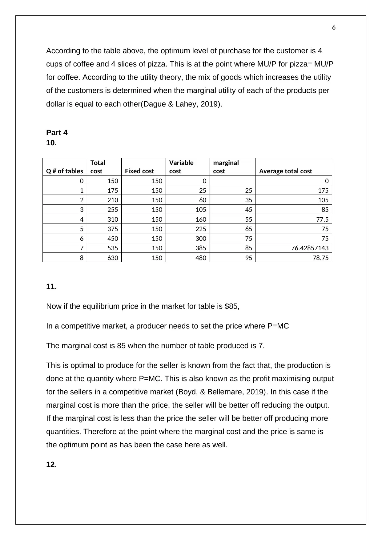
This economics assignment solution addresses several key microeconomic concepts. Part 1 analyzes the effects of rent control on the equilibrium price and quantity of rental apartments, discussing consumer and producer surplus, and deadweight loss. Part 2 examines the impact of taxes on both the apartment and luxury watch markets, detailing consumer and producer surplus, deadweight loss, and tax revenue. Part 3 delves into consumer choice theory, determining optimal purchases using budget lines, total and marginal utility, and the marginal utility per dollar. Finally, Part 4 explores cost structures, marginal cost, and the determination of profit-maximizing output in a competitive market, including the distinction between short-run and long-run equilibrium.

1
BUSINESS ECONOMICS ASSIGNMENT

2
Contents
Part 1............................................................................................................................3
Part 2............................................................................................................................3
Part 3............................................................................................................................4
Part 4............................................................................................................................5
Reference.....................................................................................................................7

3
Part 1
1. The equilibrium price and the quantity for the rented apartment as shown in
the figure are $1000 and 1000 units respectively. This is the point the demand
curve and the supply curve have intersected to produce the equilibrium. The
equilibrium is that point where the demand of the market is exactly equal to
the supply by the sellers (Trost, 2019).
2. As per the figure, due to the rent control at $700, there will be more demand
at the market than supply. Therefore, there will be shortage of rented
apartment in the market. The new price ceiling will intersect the supply curve
at the point where the quantity of apartment rented will be 700.
3. Now that the rent control has been in effect,
i) The consumer surplus in this case is shown by the area A+B+C. This is
the area below the demand curve and above the price. This is called
the consumer surplus as the consumers have to pay less than their
willingness to pay to the producers (Besanko & Braeutigam, 2020).
ii) The producers’ surplus in this case is shown by the area D in the
figure. This is the area above the supply curve and below the price.
This is called the producers surplus as the producers with low
willingness to supply earns a more price in this case.
iii) The dead-weight loss is shown by the area of E+F in the figure. The
dead weight loss is the social loss due to the implementation of the rent
control.
Part 2
4. Before any tax is levied, the equilibrium price and quantity in the rental
apartment market are $1000 and 1000 units respectively. The equilibrium
price and the quantity in case of the luxury watch market are $1000 and 1000
units of watch. This has been collected from the intersection of the demand
and the supply curve in both the cases (Mankiw, 2020).
5.
Tax on apartment Tax on watches
Price paid by $1300 $1200

4
consumers
Price received by
producers
$700 $600
Quantity of units sold
or rented
700 600
Total tax revenue
collected
$420000 $360000
Dead weight loss $90000 $120000
6. In the figure 1, the consumer surplus is show by the area A as this is area
below the demand curve and the price paid for the rented apartment. The
producer’s surplus is shown by the area D as this is the area above the supply
curve and below the price which is received by the seller (Jackson, 2019).
The dead weight loss in the area is shown by the area E+F. This is the area
which is not received by any agent of the society. The area shown by B+C is
the tax revenue which is collected by the government.
In the figure 2, the consumer’s surplus is shown by the area A, the area which
is below the demand curve and above the price level for the watches. The
producers’ surplus is shown by the area D, this is the area which is above the
supply curve and below the price received for the watches (Galambos, 2019).
The dead weight loss is the area shown by E+F and the revenue collected by
the government is shown by the area B+C.
Part 3
7. Among the budget lines shown in the figure 3, the line marked by the letter C
is the budget line of Anna. This is because of the fact that Anna’s budget is
$24 and the price of each slices of pizza is $4 (Taylor, 2019). That means if
she buys only slices of pizza than she would be able to buy 6 scales of pizza.
Therefore, given the number of slices of pizza in the horizontal axis, 6 should
be the intercept, which is same in case of the budget line shown by the letter
C. Again, if she had bought only cups of coffee with the whole money, she
could have bought 12 cups of coffee. The curve C intersects the vertical Axis
exactly in the point of 12. Therefore, this curve is the accurate one as per the
information provided.

5
8.
Pizza # of slices Total utility Marginal utility MU per dollar
1 72 72 18
2 140 68 17
3 204 64 16
4 264 60 15
5 320 56 14
6 372 52 13
7 420 48 12
8 464 44 11
Coffee # of cups Total utility Marginal utility MU per dollar
1 45 45 22.5
2 85 40 20
3 120 35 17.5
4 150 30 15
5 175 25 12.5
6 195 20 10
7 210 15 7.5
8 220 10 5
9.
Which one is
purchased
Purchas
e #
Pizza
MU/P
Coffee
MU/P Pizza Coffee
Amount spent on
purchase
Total amount
spent
1 18 22.5 ✓ $2 $24
2 17 20 ✓ $4 $24
3 16 17.5 ✓ $6 $24
4 15 15 ✓ ✓ $8 $24
5 14 12.5 ✓ $10 $24
6 13 10 ✓ $12 $24
7 12 7.5 ✓ $14 $24
8 11 5 ✓ $32 $24
9
10
Total 116 110

6
According to the table above, the optimum level of purchase for the customer is 4
cups of coffee and 4 slices of pizza. This is at the point where MU/P for pizza= MU/P
for coffee. According to the utility theory, the mix of goods which increases the utility
of the customers is determined when the marginal utility of each of the products per
dollar is equal to each other(Dague & Lahey, 2019).
Part 4
10.
Q # of tables
Total
cost Fixed cost
Variable
cost
marginal
cost Average total cost
0 150 150 0 0
1 175 150 25 25 175
2 210 150 60 35 105
3 255 150 105 45 85
4 310 150 160 55 77.5
5 375 150 225 65 75
6 450 150 300 75 75
7 535 150 385 85 76.42857143
8 630 150 480 95 78.75
11.
Now if the equilibrium price in the market for table is $85,
In a competitive market, a producer needs to set the price where P=MC
The marginal cost is 85 when the number of table produced is 7.
This is optimal to produce for the seller is known from the fact that, the production is
done at the quantity where P=MC. This is also known as the profit maximising output
for the sellers in a competitive market (Boyd, & Bellemare, 2019). In this case if the
marginal cost is more than the price, the seller will be better off reducing the output.
If the marginal cost is less than the price the seller will be better off producing more
quantities. Therefore at the point where the marginal cost and the price is same is
the optimum point as has been the case here as well.
12.

7
The market price of $85 is not the long run equilibrium price as in the long run the
seller cannot make supernormal profit. In this case, the difference between the level
of price and the average total cost is the economic profit earned by the seller in the
long run (Jullien, Stol & Herbsleb, 2019). In the long run there will be no difference
between the marginal cost, price and the average total cost of production. This will
happen when the marginal cost will be 75 which are equal to the average total cost
at this production level (Ficano, 2019). Therefore the long run equilibrium price is
$75 and the quantity is 6 numbers of tables.

8
Reference
Besanko, D., & Braeutigam, R. (2020). Microeconomics. John Wiley & Sons.
Boyd, C. M., & Bellemare, M. F. (2019). The Microeconomics of Agricultural Price
Risk, 16(1), 125-130.
Dague, L., & Lahey, J. N. (2019). Causal inference methods: Lessons from applied
microeconomics. Journal of Public Administration Research and Theory,
29(3), 511-529.
Ficano, C. K. C. (2019). Identifying differential benefits from a flipped-group
pedagogy in introductory microeconomics. International Review of Economics
Education, 30, 100143.
Galambos, L. (2019). Taylor, Jason E. Deconstructing the Monolith: The
Microeconomics of the National Industrial Recovery Act. Chicago: University
of Chicago Press, 2019. Essays in Economic & Business History, 37, 249-
251.
Jackson, D. H. (2019). The microeconomics of the timber industry. Routledge.
Jullien, N., Stol, K. J., & Herbsleb, J. D. (2019). A Preliminary Theory for Open-
Source Ecosystem Microeconomics. In Towards Engineering Free/Libre Open
Source Software (FLOSS) Ecosystems for Impact and Sustainability (pp. 49-
68). Springer, Singapore.
Mankiw, N. G. (2020). Principles of microeconomics. Cengage Learning.
Taylor, J. E. (2019). Deconstructing the monolith: The microeconomics of the
national industrial recovery act. University of Chicago Press.
Trost, B. (2019). Essays in Applied Microeconomics: Topics in Urban and Education
Economics.