Analysis of Fluid Friction in Pipes: MECH202 Lab 4 Experiment Report

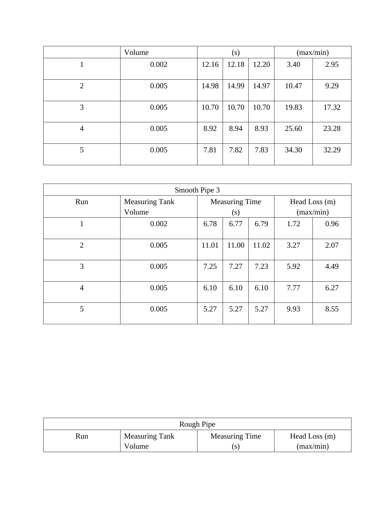
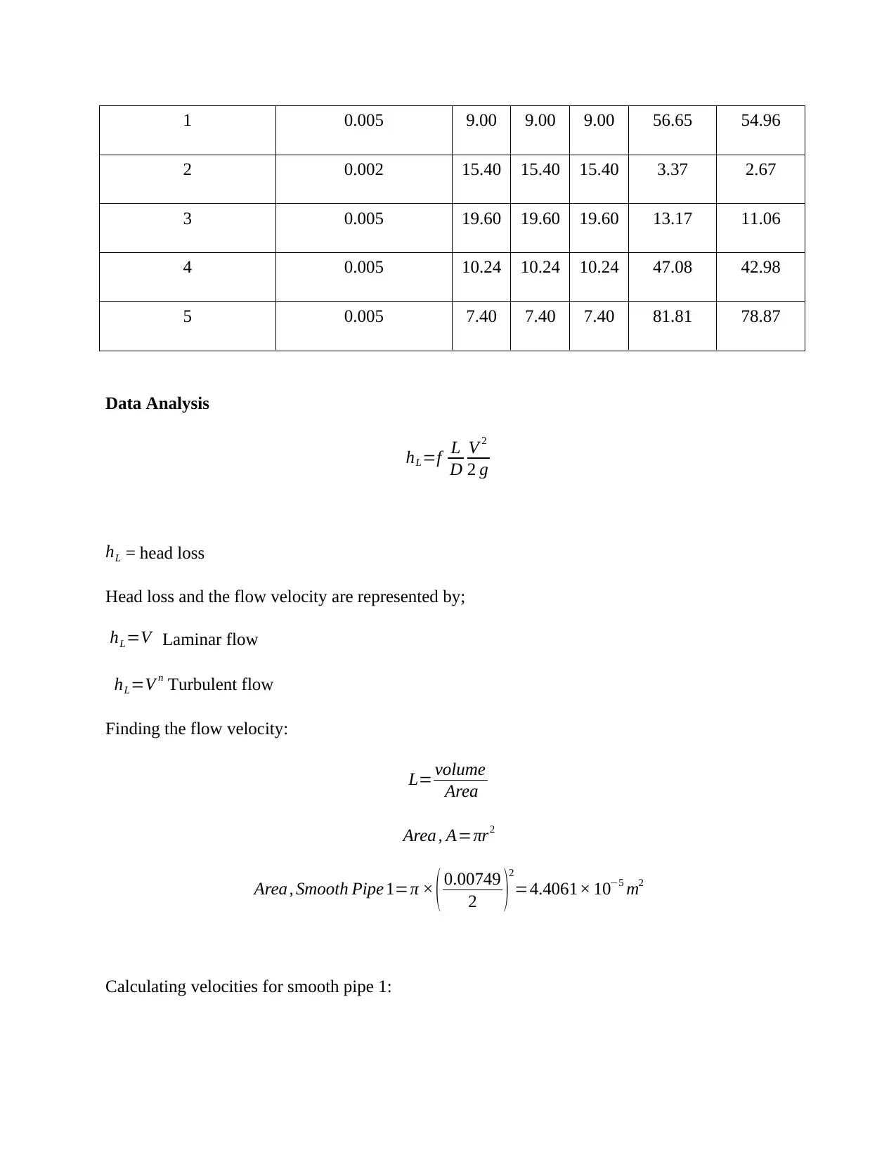
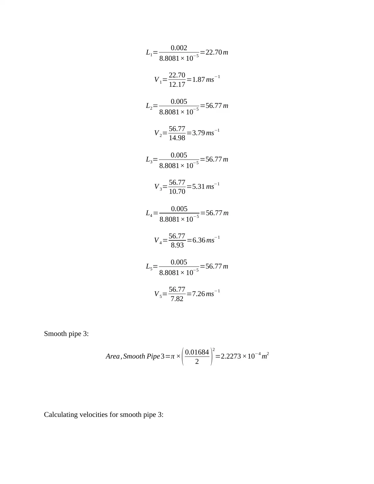
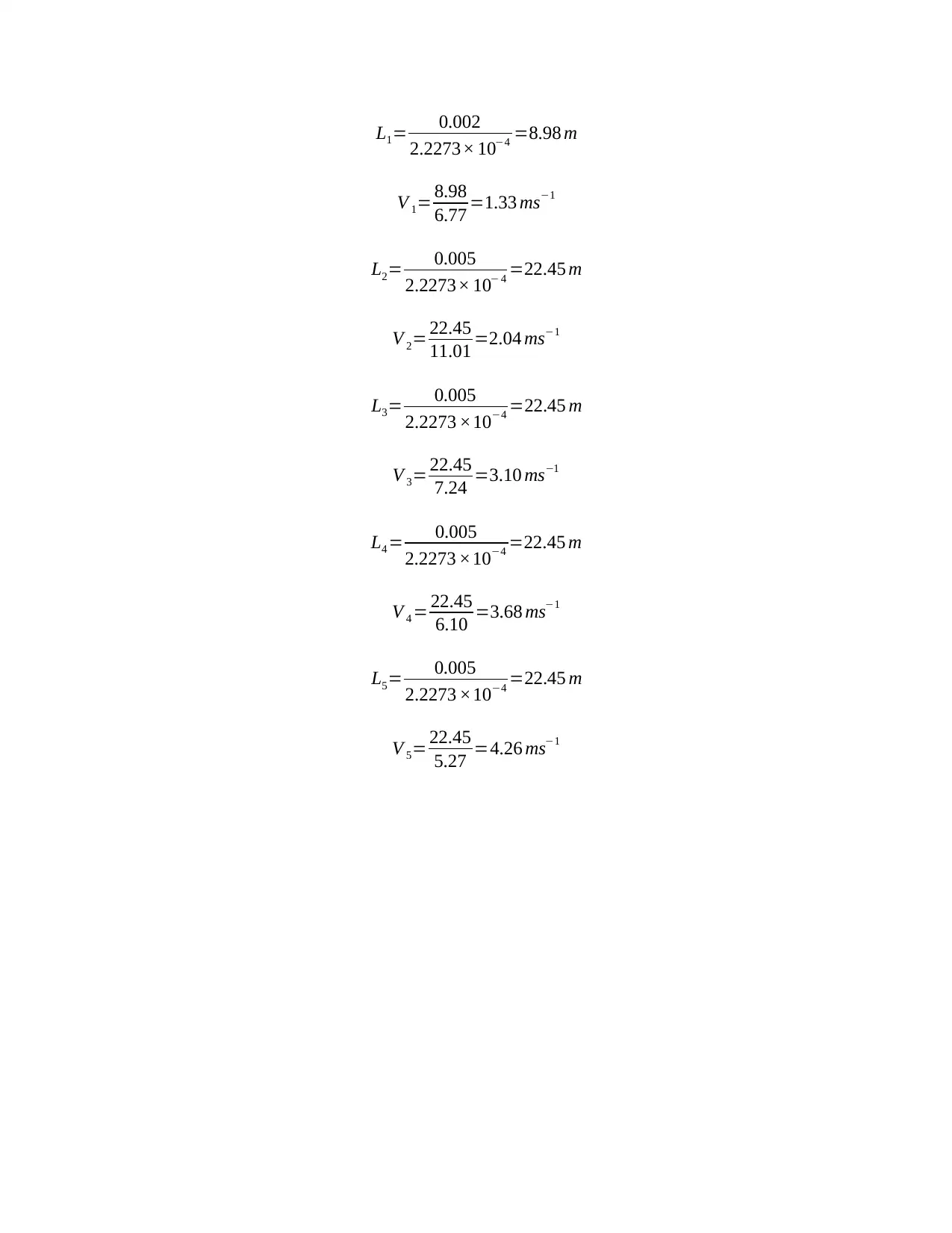
This lab report investigates fluid friction in pipes, focusing on the relationship between head loss and fluid velocity in both smooth and rough pipes. The experiment involves measuring head losses at various flow rates, calculating flow velocities, and determining the friction factor. The report includes detailed data analysis, calculations of Reynolds numbers, and comparisons between measured and calculated head losses. Graphs of head loss versus flow velocity are presented, and the results are discussed in relation to laminar and turbulent flow regimes. The report also estimates pipe roughness using the Moody diagram and experimental data, highlighting the impact of friction on energy loss in fluid flow systems. The conclusion summarizes the key findings and acknowledges potential sources of error.

INSTITUTION
NAME
REGISTRATION NO:
COURSE
PROFESSORS NAME:
EXPERIMENT: Lab 4 Fluid friction in pipes
DATE

Objectives
 Determine relationship between the head loss and fluid velocity.
 Express the relationship that exists between the head loss and flow velocity.
 Make a comparison between the calculated and the measured and head losses.
 To determine pipe roughness.
Introduction
The main purpose of this experiment’s was to investigate relationship between the head losses
and the velocity of flow. Head losses are caused by fluid friction. It was done with respect to
both a smooth and rough test pipes. This was achieved after establishing the relationship that
existed between the head loss and flow velocity. Relationship was used in comparing the
measured head loss and calculated head loss. The unknown pipe roughness was also established.
Theory
A fluid experiences some resistance when flowing through a pipe. This is due to the shear
stresses that convert fraction of the fluid’s energy into a loss and it is known as head loss which
is a product of friction and it is a function of the pipe’s length, diameter, mean flow velocity,
fluid’s property and actual pipe roughness. An important note is that head loss as a result of
friction is independent of the fluid flow pressure, in this case water [1].
Mathematical expression of the relationship between head loss and flow velocity:
hL=f L
D
V 2
2 g
Where:
hL=head loss due ¿ friction( m)
f =friction

L=length of pipe(m)
D=diameter of pipe(m)
V =average flow velocity (ms−1 )
g=acceleration due ¿ gravity (ms−2 )
Measurement and determination of the pipes head losses can be done by considering a given
range of Reynolds’ number. These numbers are what determine if a pipe flow is laminar,
transitional or turbulent. A smooth pipe and a roughened test pipe are used.
Relationship between head loss and flow velocity [2]:
hL ≈ V for laminar flow
hL ≈ for turbulent flow
In transitional flow, it is challenging to determine the effects of fluid friction that can cause head
losses and establish its relationship with the flow velocity.
Apparatus
 Fluid friction apparatus.
 Hydraulic Bench.
 Portable pressure meter.
 Volumetric tank.
 Measuring cylinder.
 Vernier Calipers.
Procedure

 Priming of the pipe network was done until air appeared not to be discharged from the
apparatus.
 Valves were opened and closed and water flow was obtained through the required test
pipe where four lowest pipes of fluid friction apparatus were used.
 Head losses between the tappings were measured by portable pressure meter for five
different flow rates achieved by altering the flow on the control valve of the hydraulics
bench of each pipe.
 The internal diameter of individual test pipe was then measured using a Vernier caliper.
 The results were recorded in a tabular form.
Data
Smooth Pipe 1 Smooth Pipe 2 Smooth Pipe 3 Rough Pipe
Diameter (m) 0.00749 0.01059 0.01684 0.01684
Smooth Pipe 1
Run Measuring Tank
Volume
Measuring Time
(s)
Head Loss (m)
(max/min)
1 0.002 15.45 15.44 15.43 11.31 10.47
2 0.002 9.40 9.40 9.40 32.16 31.21
3 0.005 14.40 14.40 14.40 73.44 71.08
4 0.005 13.24 13.24 13.24 77.25 74.62
5 0.005 10.60 10.60 10.60 79.60 76.82
Smooth Pipe 2
Run Measuring Tank Measuring Time Head Loss (m)

Volume (s) (max/min)
1 0.002 12.16 12.18 12.20 3.40 2.95
2 0.005 14.98 14.99 14.97 10.47 9.29
3 0.005 10.70 10.70 10.70 19.83 17.32
4 0.005 8.92 8.94 8.93 25.60 23.28
5 0.005 7.81 7.82 7.83 34.30 32.29
Smooth Pipe 3
Run Measuring Tank
Volume
Measuring Time
(s)
Head Loss (m)
(max/min)
1 0.002 6.78 6.77 6.79 1.72 0.96
2 0.005 11.01 11.00 11.02 3.27 2.07
3 0.005 7.25 7.27 7.23 5.92 4.49
4 0.005 6.10 6.10 6.10 7.77 6.27
5 0.005 5.27 5.27 5.27 9.93 8.55
Rough Pipe
Run Measuring Tank
Volume
Measuring Time
(s)
Head Loss (m)
(max/min)

1 0.005 9.00 9.00 9.00 56.65 54.96
2 0.002 15.40 15.40 15.40 3.37 2.67
3 0.005 19.60 19.60 19.60 13.17 11.06
4 0.005 10.24 10.24 10.24 47.08 42.98
5 0.005 7.40 7.40 7.40 81.81 78.87
Data Analysis
hL=f L
D
V 2
2 g
hL = head loss
Head loss and the flow velocity are represented by;
hL=V Laminar flow
hL=V n Turbulent flow
Finding the flow velocity:
L= volume
Area
Area , A=πr2
Area , Smooth Pipe 1=π × ( 0.00749
2 )
2
=4.4061× 10−5 m2
Calculating velocities for smooth pipe 1:

L1= 0.002
4.4061 ×10−5 =45.39 m
V 1= 45.39
15.45 =2.94 ms−1
L2= 0.002
4.4061 ×10−5 =45.39 m
V 2= 45.39
9.395 =4.83 ms−1
L3= 0.005
4.4061 ×10−5 =113.48 m
V 3= 113.48
14.40 =7.88 ms−1
L4 = 0.005
4.4061× 10−5 =113.48 m
V 4 =113.48
13.25 =8.56 ms−1
L5= 0.005
4.4061 ×10−5 =113.48 m
V 5= 113.48
10.60 =10.71 ms−1
Smooth pipe 2:
Area, Smooth Pipe 2=π × ( 0.01059
2 )
2
=8.8081×10−5 m2
Calculating velocities for smooth pipe 2:

L1= 0.002
8.8081× 10−5 =22.70 m
V 1= 22.70
12.17 =1.87 ms−1
L2= 0.005
8.8081× 10−5 =56.77 m
V 2= 56.77
14.98 =3.79 ms−1
L3= 0.005
8.8081× 10−5 =56.77 m
V 3= 56.77
10.70 =5.31 ms−1
L4 = 0.005
8.8081×10−5 =56.77 m
V 4 =56.77
8.93 =6.36 ms−1
L5= 0.005
8.8081× 10−5 =56.77 m
V 5= 56.77
7.82 =7.26 ms−1
Smooth pipe 3:
Area, Smooth Pipe 3=π × ( 0.01684
2 )
2
=2.2273 ×10−4 m2
Calculating velocities for smooth pipe 3:

L1= 0.002
2.2273× 10−4 =8.98 m
V 1= 8.98
6.77 =1.33 ms−1
L2= 0.005
2.2273× 10− 4 =22.45 m
V 2= 22.45
11.01 =2.04 ms−1
L3= 0.005
2.2273 ×10−4 =22.45 m
V 3= 22.45
7.24 =3.10 ms−1
L4 = 0.005
2.2273 ×10−4 =22.45 m
V 4 = 22.45
6.10 =3.68 ms−1
L5= 0.005
2.2273 ×10−4 =22.45 m
V 5= 22.45
5.27 =4.26 ms−1

Discussion
Graphs 1 &2 of Head Loss verses Flow Velocity
0.4 0.5 0.6 0.7 0.8 0.9 1 1.1
0
0.2
0.4
0.6
0.8
1
1.2
1.4
1.6
1.8
2 f(x) = 1.59741315608799 x + 0.361675166186216
R² = 0.956207143014561
Smooth Pipe 1
Smooth Pipe 1 Linear (Smooth Pipe 1) Linear (Smooth Pipe 1)
Log V
Log hL
From:
hL=V n
Therefore, log ( hL ) =nlog ( V ) + log (c)
But, y=mx+c
y = 1.5974x + 0.3617
n=1.5974
A turbulent type of flow is expected to be created by the flow rate.

0.2 0.3 0.4 0.5 0.6 0.7 0.8 0.9
0
0.2
0.4
0.6
0.8
1
1.2
1.4
1.6
1.8
f(x) = 1.69187176987238 x + 0.0621409305580984
R² = 0.998328012704899
Smooth Pipe 2
Smooth Pipe 2 Linear (Smooth Pipe 2)
Log V
Log hL
From:
hL=V n
Therefore, log ( hL ) =nlog ( V ) + log (c)
But, y=mx+c
y = 1.6919x + 0.0621
n=1.6919
A turbulent type of flow is expected from the flow rate.
.

0 0.1 0.2 0.3 0.4 0.5 0.6 0.7
0
0.2
0.4
0.6
0.8
1
1.2
f(x) = 1.49114439233679 x + 0.0496449547613562
R² = 0.999476124745447
Smooth Pipe 3
Smooth Pipe 3 Linear (Smooth Pipe 3) Linear (Smooth Pipe 3)
Log V
Log hL
From:
hL=V n
Therefore, log ( hL ) =nlog ( V ) + log (c)
But, y=mx+c
y = 1.4911x + 0.0496
n=1.4911
A transitional type of flow is expected to be created from the flow rate.