BUS5SBF: Statistics for Business and Finance - Household Data Analysis

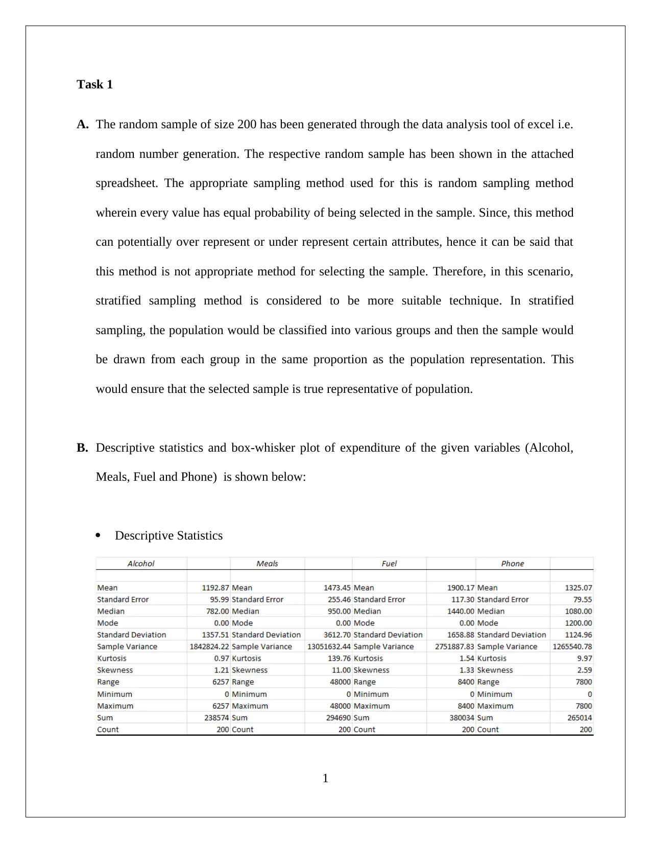
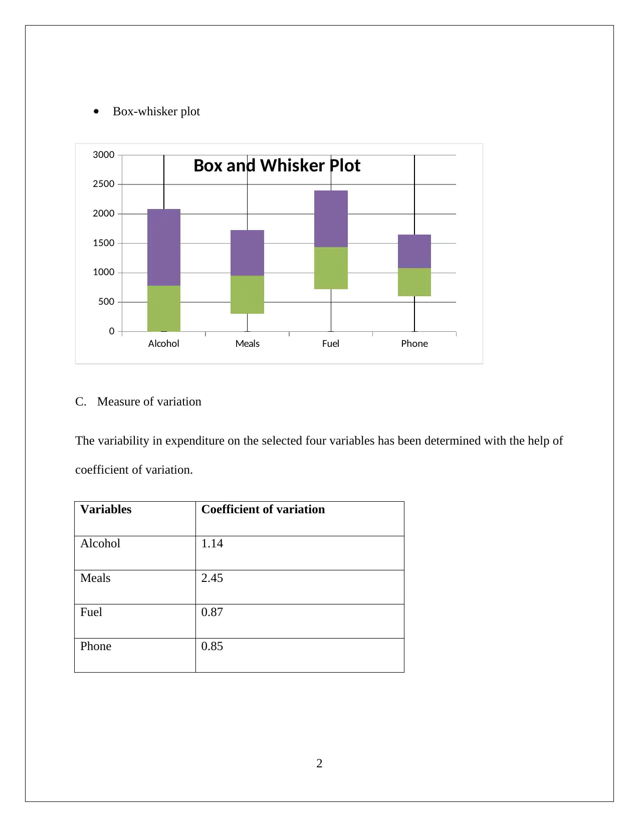
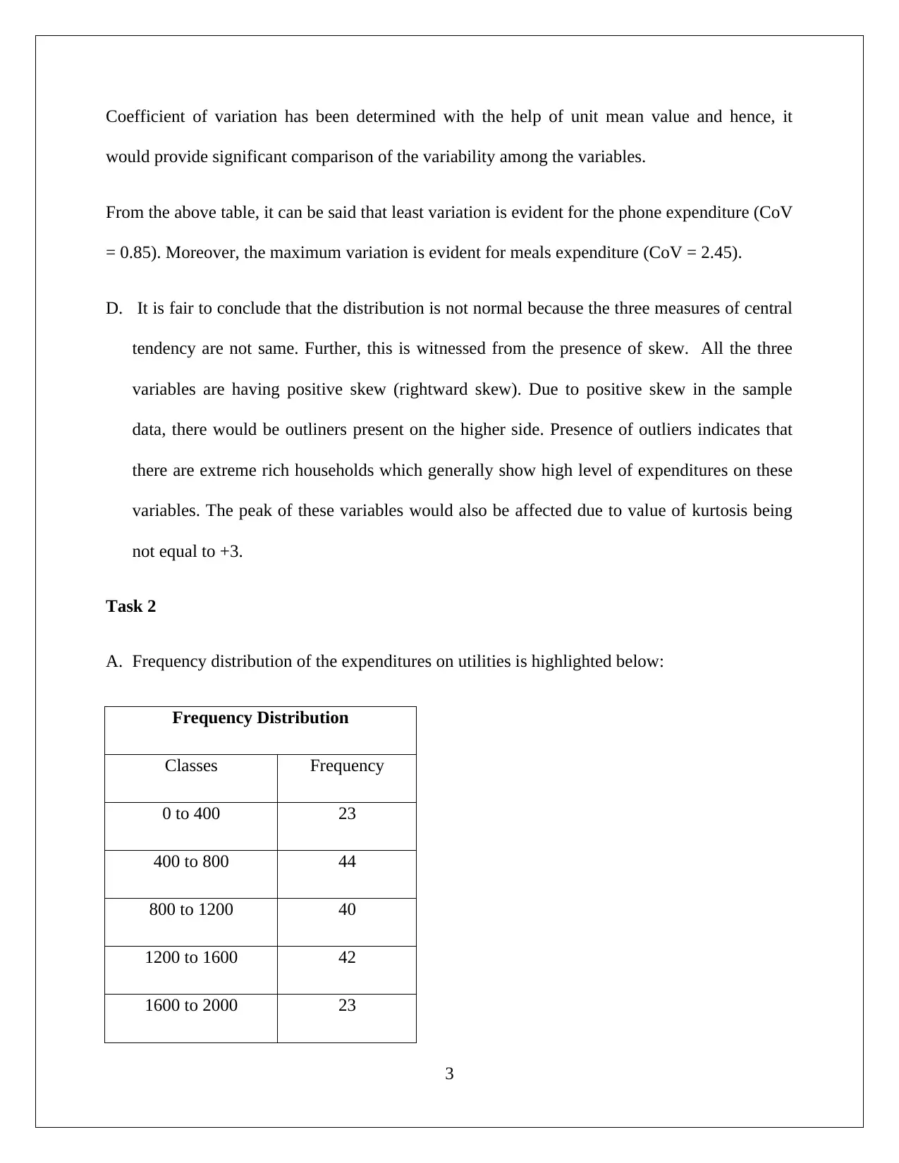
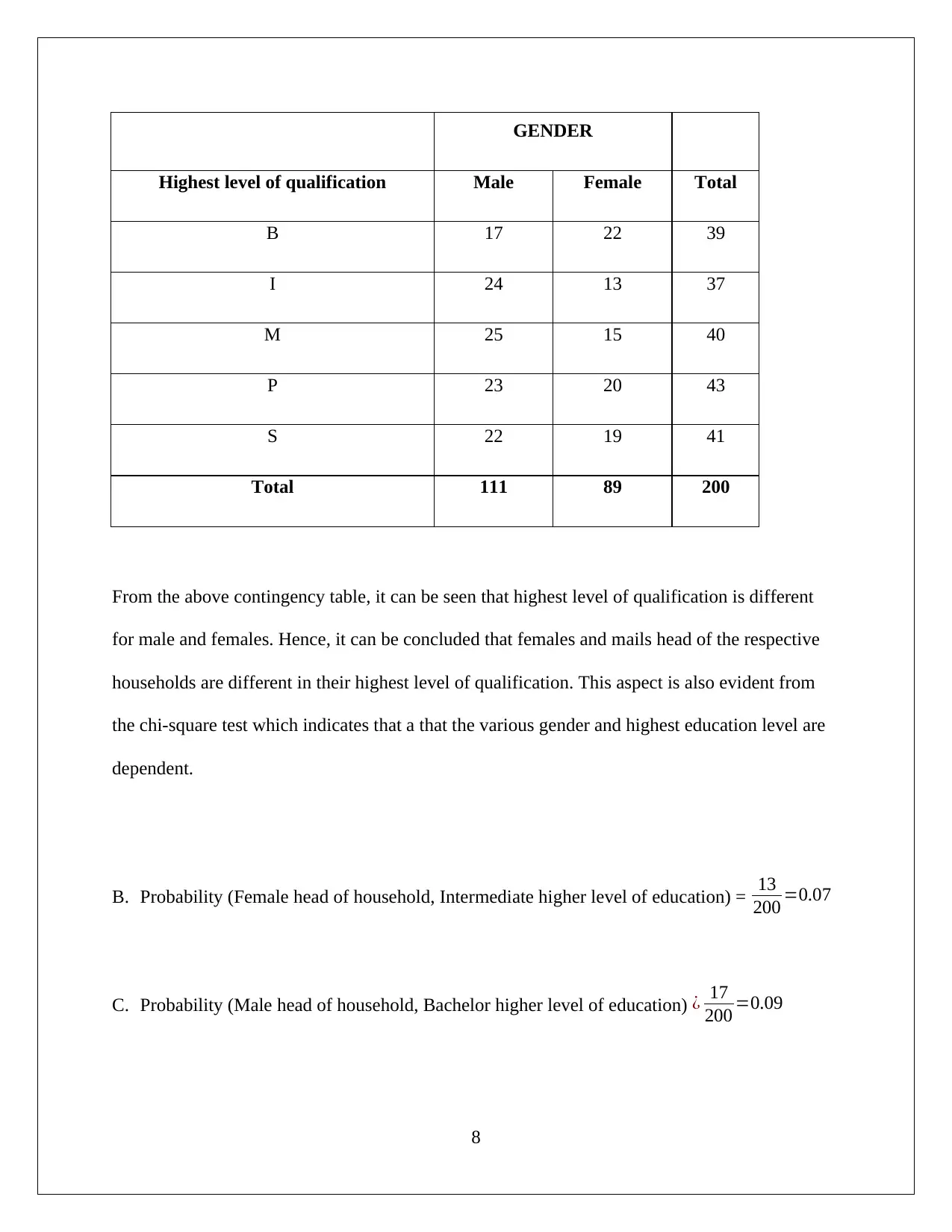
This document presents a comprehensive analysis of household data, addressing various statistical concepts and techniques. The analysis begins with a discussion of sampling methods, comparing random and stratified sampling, and justifying the use of stratified sampling. Descriptive statistics, including measures of variation (coefficient of variation) and box-whisker plots, are used to analyze the expenditure on variables like alcohol, meals, fuel, and phone. The assignment also explores frequency distributions and histograms for utility expenditures, identifying the distribution's characteristics. Furthermore, the document investigates income disparities by comparing the top and bottom 10% of household after-tax income and examines the relationship between after-tax income and total expenditure using correlation and scatter plots. Finally, a contingency table is constructed to analyze the relationship between gender and education levels, and the independence of events is tested using probability calculations and chi-square tests. The analysis provides insights into household characteristics, income distribution, and relationships between variables, demonstrating a strong understanding of statistical concepts.

STATISTICS FOR BUSINESS AND FINANCE (BUS5SBF)
Analyzing Household Data
[Pick the date]
STUDENT ID

Task 1
A. The random sample of size 200 has been generated through the data analysis tool of excel i.e.
random number generation. The respective random sample has been shown in the attached
spreadsheet. The appropriate sampling method used for this is random sampling method
wherein every value has equal probability of being selected in the sample. Since, this method
can potentially over represent or under represent certain attributes, hence it can be said that
this method is not appropriate method for selecting the sample. Therefore, in this scenario,
stratified sampling method is considered to be more suitable technique. In stratified
sampling, the population would be classified into various groups and then the sample would
be drawn from each group in the same proportion as the population representation. This
would ensure that the selected sample is true representative of population.
B. Descriptive statistics and box-whisker plot of expenditure of the given variables (Alcohol,
Meals, Fuel and Phone) is shown below:
 Descriptive Statistics
1

 Box-whisker plot
Alcohol Meals Fuel Phone
0
500
1000
1500
2000
2500
3000
Box and Whisker Plot
C. Measure of variation
The variability in expenditure on the selected four variables has been determined with the help of
coefficient of variation.
Variables Coefficient of variation
Alcohol 1.14
Meals 2.45
Fuel 0.87
Phone 0.85
2

Coefficient of variation has been determined with the help of unit mean value and hence, it
would provide significant comparison of the variability among the variables.
From the above table, it can be said that least variation is evident for the phone expenditure (CoV
= 0.85). Moreover, the maximum variation is evident for meals expenditure (CoV = 2.45).
D. It is fair to conclude that the distribution is not normal because the three measures of central
tendency are not same. Further, this is witnessed from the presence of skew. All the three
variables are having positive skew (rightward skew). Due to positive skew in the sample
data, there would be outliners present on the higher side. Presence of outliers indicates that
there are extreme rich households which generally show high level of expenditures on these
variables. The peak of these variables would also be affected due to value of kurtosis being
not equal to +3.
Task 2
A. Frequency distribution of the expenditures on utilities is highlighted below:
Frequency Distribution
Classes Frequency
0 to 400 23
400 to 800 44
800 to 1200 40
1200 to 1600 42
1600 to 2000 23
3

2000 to 2400 10
2400 to 2800 8
2800 to 3200 6
More than 3200 4
Total 200
B. Percentage of households that spend on utilities is computed based on the frequency
distribution.
At themost $ 1200 per annum=23+ 44+ 40
200 =0.53∨53.5 %
Between $ 1200∧$ 2400 per annum= 42+23+10
200 =0.375∨37.5 %
More than $ 2400 per annum= 8+6+4
200 =0.09∨9 %
D. Histogram for the expenditure on utilities is shown below:
4

0 to 400 400 to
800 800 to
1200 1200 to
1600 1600 to
2000 2000 to
2400 2400 to
2800 2800 to
3200 More
than
3200
0
5
10
15
20
25
30
35
40
45
50
Histogram - Utility
Expenditure on utility ($)
Frequency
From the above histogram, it can be said that distribution is not normal. Moreover, the long right
side tail in histogram indicates presence of rightward skew.
Task 3
A. The respective top and bottom 10% of household after tax income (ataxInc) is computed in
excel and highlighted below:
Top 10% value of household ataxInc 99719.5
Bottom 10% value of household ataxInc 17032.4
5

This indicates the difference in the income levels of society. Moreover, the top 10 % value of
household after tax income indicates the richest part of society. While, the bottom 10% value of
household after tax income indicates the poorest part of society.
B. The mean of variable OwnHouse is 0.745, implies that nearly 74.5% of the houses are used
by their owners themselves only, while the rest of 25.5% have been extended to tenants for
rent purposes.
C. The probability that a randomly selected household will have a family size of 5 is computed
below:
Total sample = 200,
Number of sample which is having family size (child +Adult) of 5 = 12
Probability ¿ 12
200 =0.06
D. Scatter plot for ln (ataxlnc)vs ln(texp) is shown below:
6

8 10 12 14
0
2
4
6
8
10
12
14
Scatter Plot
ln (ATaxInc)
ln ((Texp)
Coefficient of correlation is determined with the help of CORREL function of excel. The value
of coefficient of correlation is 0.66.
It can be seen from the scatter plot and correlation coefficient that variables after tax income and
total expenditure are showing a positive linear relationship. It means those who have high level
of after tax income would also tend to display a high level of total expenditure. Further, it is
noteworthy that as the value of correlation coefficient is not closer to 1 and hence, it can be said
that these variables are not having strong linear relationship.
Task 4
A. Construction of contingency table between the variables gender and level of education is
shown below:
Contingency Table
7

GENDER
Highest level of qualification Male Female Total
B 17 22 39
I 24 13 37
M 25 15 40
P 23 20 43
S 22 19 41
Total 111 89 200
From the above contingency table, it can be seen that highest level of qualification is different
for male and females. Hence, it can be concluded that females and mails head of the respective
households are different in their highest level of qualification. This aspect is also evident from
the chi-square test which indicates that a that the various gender and highest education level are
dependent.
B. Probability (Female head of household, Intermediate higher level of education) = 13
200 =0.07
C. Probability (Male head of household, Bachelor higher level of education) ¿ 17
200 =0.09
8