University Project: Organic Food Expenditure Analysis and Regression

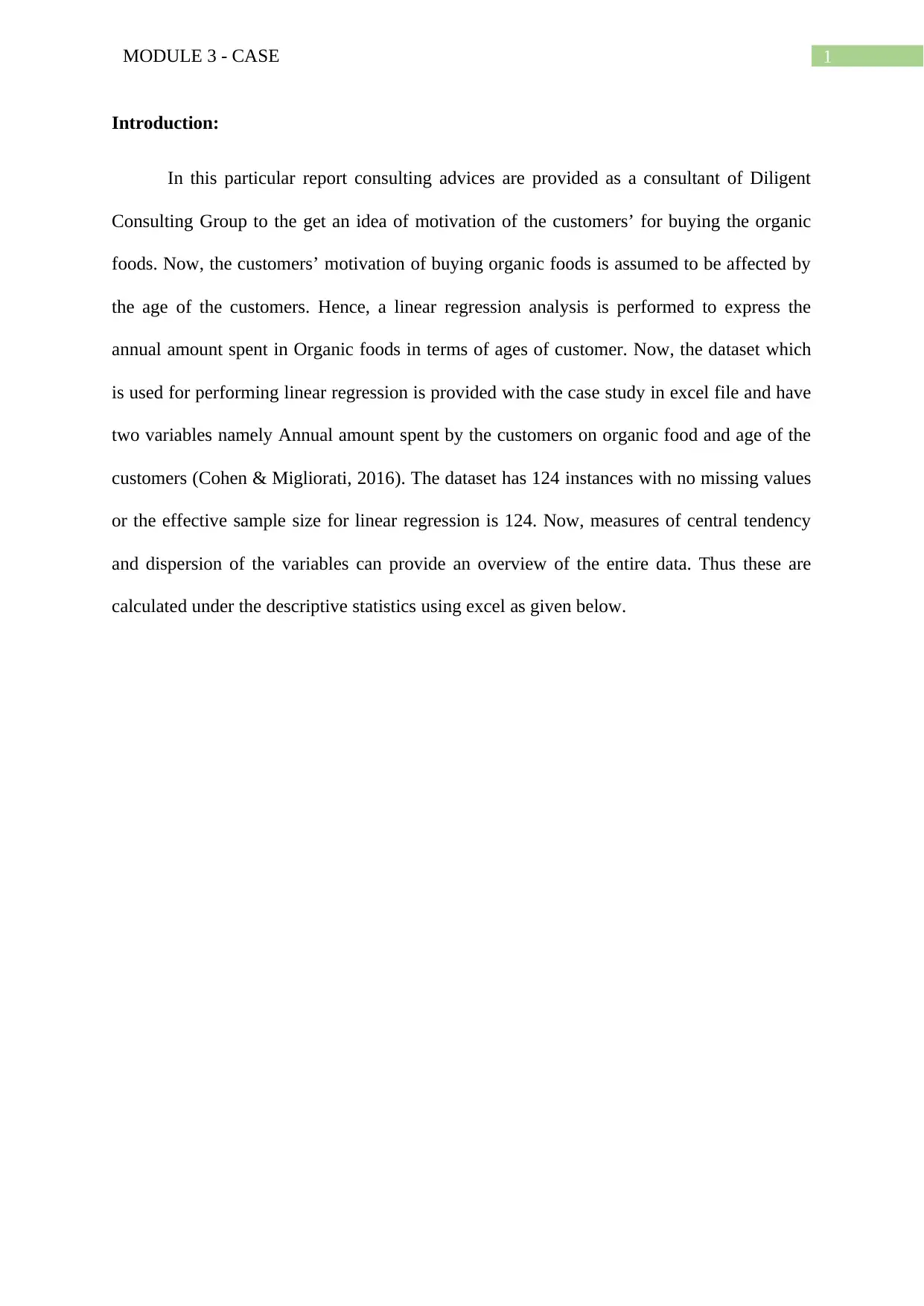
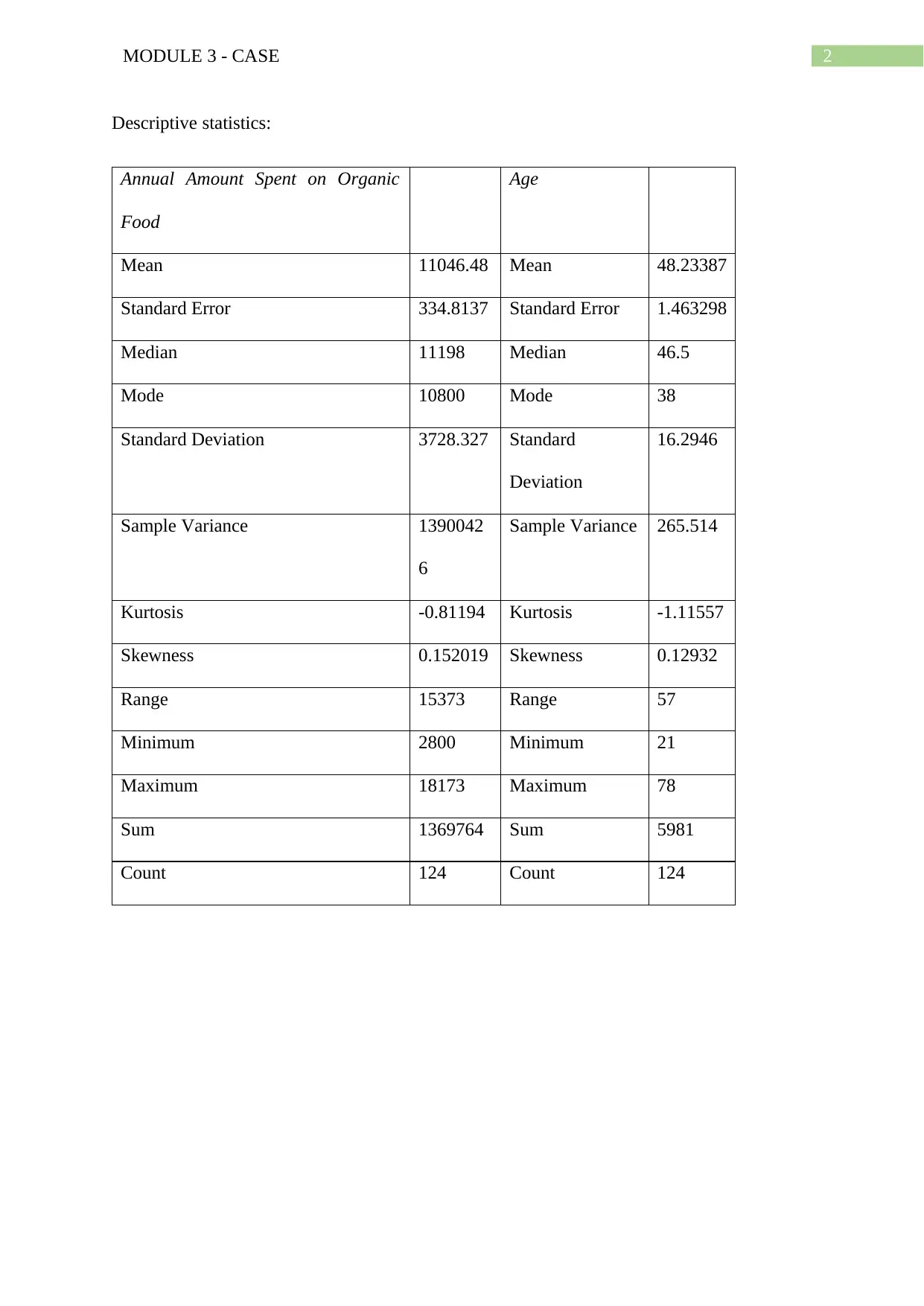
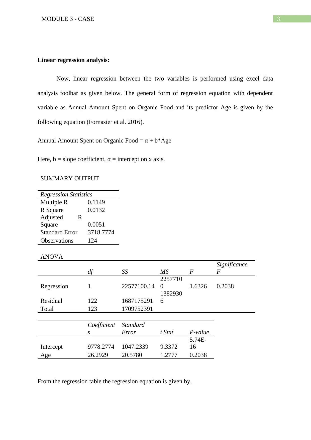
This report presents a linear regression analysis conducted to understand the relationship between customer age and their annual spending on organic food. The analysis, performed using an Excel dataset with 124 instances, includes descriptive statistics, regression equation derivation, and interpretation. The regression model aims to predict the annual amount spent on organic food based on customer age. The results indicate that the coefficient of determination is very low, and the overall significance level suggests the model is not suitable for predicting organic food expenditure based on age. The report concludes by advising against using the model for prediction and recommends collecting data on other relevant variables to improve the analysis. The student suggests considering non-linear or other regression types and increasing the sample size for more accurate results.

Running head: MODULE 3 - CASE
MODULE 3 - CASE
Name of the Student
Name of the University
Author Note

1MODULE 3 - CASE
Introduction:
In this particular report consulting advices are provided as a consultant of Diligent
Consulting Group to the get an idea of motivation of the customers’ for buying the organic
foods. Now, the customers’ motivation of buying organic foods is assumed to be affected by
the age of the customers. Hence, a linear regression analysis is performed to express the
annual amount spent in Organic foods in terms of ages of customer. Now, the dataset which
is used for performing linear regression is provided with the case study in excel file and have
two variables namely Annual amount spent by the customers on organic food and age of the
customers (Cohen & Migliorati, 2016). The dataset has 124 instances with no missing values
or the effective sample size for linear regression is 124. Now, measures of central tendency
and dispersion of the variables can provide an overview of the entire data. Thus these are
calculated under the descriptive statistics using excel as given below.

2MODULE 3 - CASE
Descriptive statistics:
Annual Amount Spent on Organic
Food
Age
Mean 11046.48 Mean 48.23387
Standard Error 334.8137 Standard Error 1.463298
Median 11198 Median 46.5
Mode 10800 Mode 38
Standard Deviation 3728.327 Standard
Deviation
16.2946
Sample Variance 1390042
6
Sample Variance 265.514
Kurtosis -0.81194 Kurtosis -1.11557
Skewness 0.152019 Skewness 0.12932
Range 15373 Range 57
Minimum 2800 Minimum 21
Maximum 18173 Maximum 78
Sum 1369764 Sum 5981
Count 124 Count 124

3MODULE 3 - CASE
Linear regression analysis:
Now, linear regression between the two variables is performed using excel data
analysis toolbar as given below. The general form of regression equation with dependent
variable as Annual Amount Spent on Organic Food and its predictor Age is given by the
following equation (Fornasier et al. 2016).
Annual Amount Spent on Organic Food = α + b*Age
Here, b = slope coefficient, α = intercept on x axis.
SUMMARY OUTPUT
Regression Statistics
Multiple R 0.1149
R Square 0.0132
Adjusted R
Square 0.0051
Standard Error 3718.7774
Observations 124
ANOVA
df SS MS F
Significance
F
Regression 1 22577100.14
2257710
0 1.6326 0.2038
Residual 122 1687175291
1382930
6
Total 123 1709752391
Coefficient
s
Standard
Error t Stat P-value
Intercept 9778.2774 1047.2339 9.3372
5.74E-
16
Age 26.2929 20.5780 1.2777 0.2038
From the regression table the regression equation is given by,

4MODULE 3 - CASE
y = 9778.2774 + 26.2929*x
Here, y = Annual Amount Spent on Organic Food
x = Age
Interpretation of linear regression:
Thus as an interpretation of the equation the annual amount spent in expenditure is
approximately 9778.2774 when age of customers is zero (just as a theoretical case) and with
unit increase in age of customer the amount spent in organic food annually tends to increase
by 26.2929 (Stout, 2017). The equation can be used to predict the annual organic food
expenditure for a known Age of customer by simply putting the age in the equation.
Now, an average consumer of the given dataset has the age of 48.23 years. Thus a consumer
of this age is estimated to spent annually on organic food by an amount
y = 9778.2774 + 26.2929*48.23 = 11046.38
Hence, an average consumer of 48.23 years age is likely spent an amount of 11046.38 on
organic food annually by the regression model (Quintela-del-Río & Francisco-Fernández,
2017).
The coefficient of determination R2 of the model is 0.0132 which indicates that only 1.32%
of variation in amount spent in organic food annually is explained by the variation of age
(Bujang & Baharum, 2017). Thus the regression model is not a good model estimating the
organic food expenditure in terms of age which is also supported by the low value of
correlation coefficient (as given by multiple R as 0.1149). The overall significance level of
regression analysis is over 0.05 (considered significance level) and hence it can be concluded
the model is not significant for organic food expenditure prediction (Nakagawa, Johnson &

5MODULE 3 - CASE
Schielzeth, 2017). Also, the coefficient of age has the p value more than 0.05 indicating that
Age is not a significant variable for predicting Annual organic food expenditure.
Conclusion:
Hence, in conclusion it can be stated that the linear regression technique is
successfully applied to predict the Annual expenditure on organic foods by customers in
terms of their age and it is found from the analysis that Age is not a significant variable in the
prediction. Also, it is recommended that to not use the model for predicting annual
expenditure as the model is badly fitted to the data. Hence, as a consultant of Diligent
Consulting Group it is advised to collect data of other related variables to annual food
expenditure and then to conduct the analysis again to see the model explanation. The error in
fitting can also be reduced if a larger sample size is used in analysis as the random errors in
the model will be reduced. It is also advised to apply non-linear or other type of regression
with the given data to see whether explanation of the dependent variable is improved,
however, the coefficients are also needed to be significant.

6MODULE 3 - CASE
References:
Cohen, A., & Migliorati, G. (2016). Optimal weighted least-squares methods. arXiv preprint
arXiv:1608.00512.
Fornasier, M., Peter, S., Rauhut, H., & Worm, S. (2016). Conjugate gradient acceleration of
iteratively re-weighted least squares methods. Computational Optimization and
Applications, 65(1), 205-259.
Stout, D. E. (2017). Using excel 2013 for regression-based cost estimation: Part
1. Management Accounting Quarterly, 18(2).
Quintela-del-Río, A., & Francisco-Fernández, M. (2017). Excel templates: a helpful tool for
teaching statistics. The American Statistician, 71(4), 317-325.
Bujang, M. A., & Baharum, N. (2017). A simplified guide to determination of sample size
requirements for estimating the value of intraclass correlation coefficient: a review. Archives
of Orofacial Science, 12(1).
Nakagawa, S., Johnson, P. C., & Schielzeth, H. (2017). The coefficient of determination R 2
and intra-class correlation coefficient from generalized linear mixed-effects models revisited
and expanded. Journal of the Royal Society Interface, 14(134), 20170213.