Holmes Institute HA1011: Applied Quantitative Methods Assignment

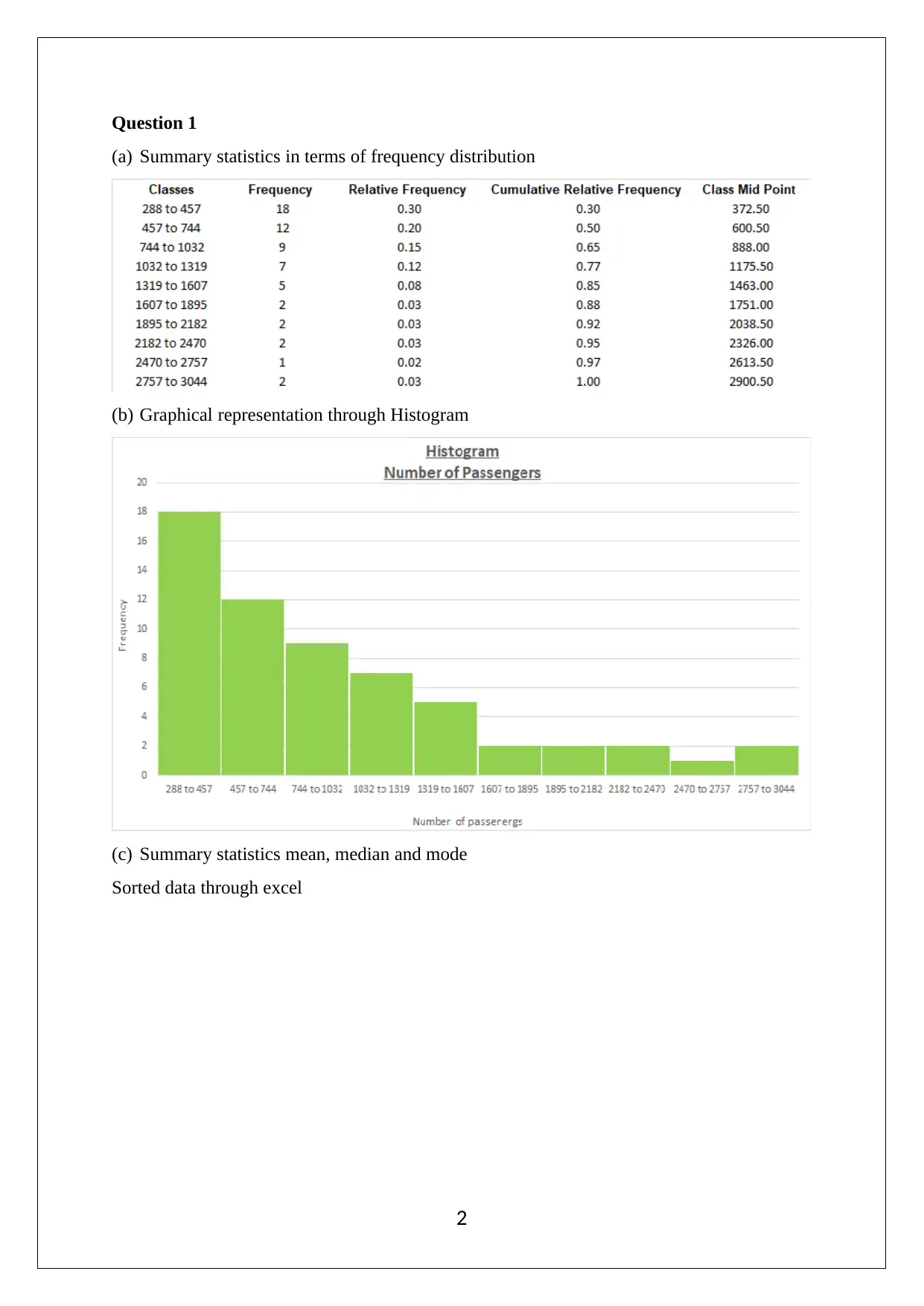
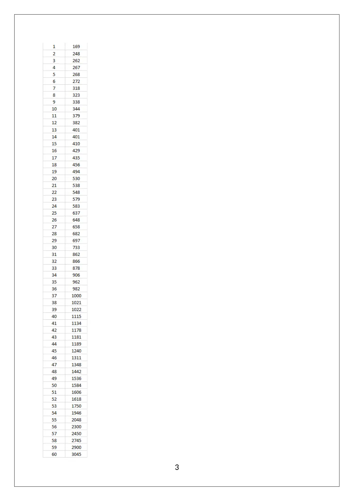
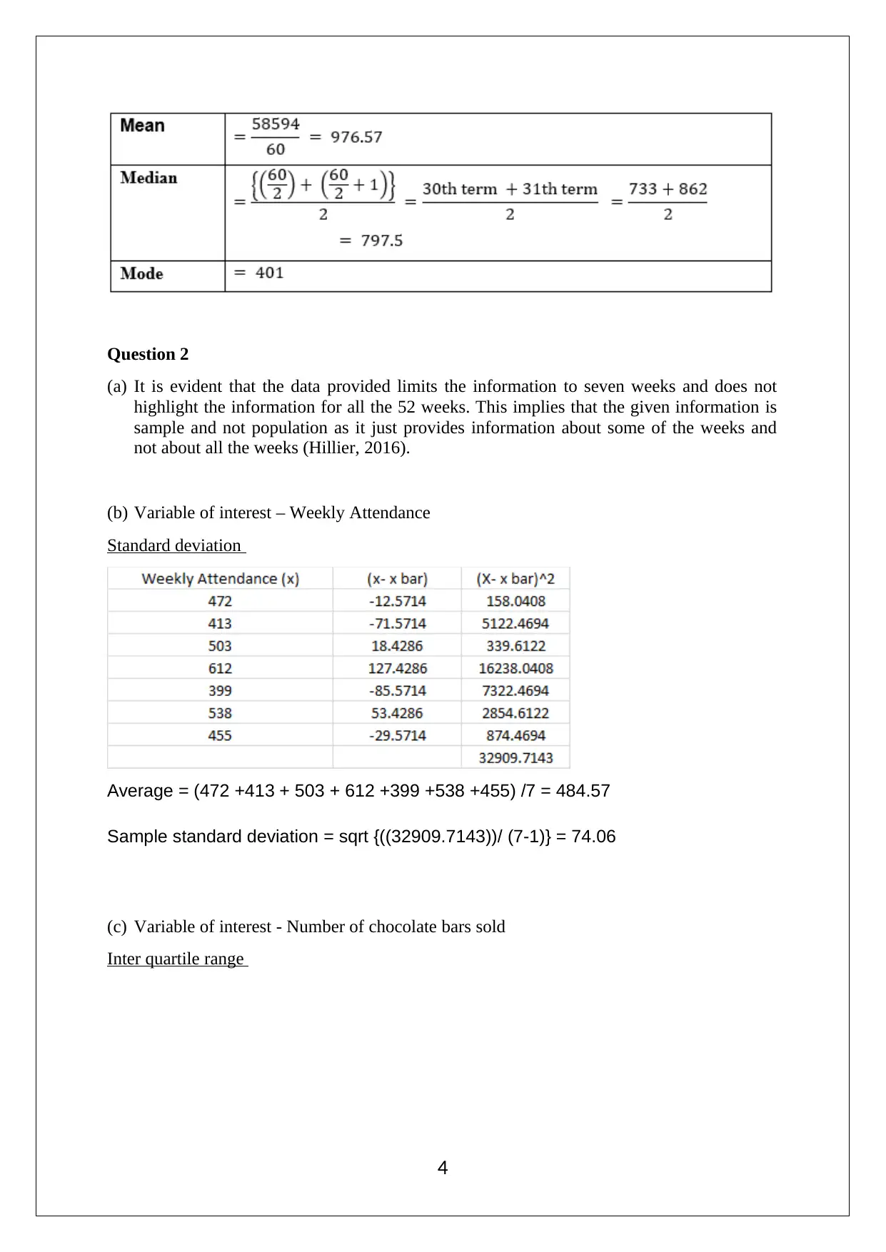
This document presents a comprehensive solution to an Applied Quantitative Methods group assignment, addressing various statistical concepts and techniques. The solution encompasses descriptive statistics, including frequency distribution, graphical representations using histograms, and measures like mean, median, and mode. It analyzes a sample dataset of weekly attendance and chocolate bar sales, calculating standard deviation, interquartile range, and correlation coefficients to understand the relationship between variables. The assignment further delves into regression analysis, deriving the least square line, interpreting its slope and intercept, and assessing the model's overall utility using the coefficient of determination. Probability concepts are explored through calculations involving independent events, conditional probabilities, and applications of binomial, Poisson, and normal distributions. The solution also addresses the Central Limit Theorem and its implications for sampling distributions. The assignment includes detailed explanations, calculations, and relevant references to support the analysis.

QUANTITATIVE METHODS
STUDENT ID:
[Pick the date]

Question 1
(a) Summary statistics in terms of frequency distribution
(b) Graphical representation through Histogram
(c) Summary statistics mean, median and mode
Sorted data through excel
2

3

Question 2
(a) It is evident that the data provided limits the information to seven weeks and does not
highlight the information for all the 52 weeks. This implies that the given information is
sample and not population as it just provides information about some of the weeks and
not about all the weeks (Hillier, 2016).
(b) Variable of interest – Weekly Attendance
Standard deviation
Average = (472 +413 + 503 + 612 +399 +538 +455) /7 = 484.57
Sample standard deviation = sqrt {((32909.7143))/ (7-1)} = 74.06
(c) Variable of interest - Number of chocolate bars sold
Inter quartile range
4

Q1 = Percentile (25th) = 25 ሺ7 + 1ሻ
100 = 2nd term = 6014
Q3 = Percentile (75th) = 75 ሺ7 + 1ሻ
100 = 6th term = 7223
IQR = Q3 − Q1 = Percentile ሺ75thሻ− Percentile ሺ25thሻ= 1209
IQR is more useful than standard deviation when the objective is to represent the dispersion
in a dataset where significant degree of skew is present and hence outliers are present. These
tend to adversely impact the accuracy of standard deviation ( Medhi, 2016).
(d) Association between variables – Correlation coefficient
The correlation coefficient is positive which implies that as the increase in weekly attendance
is witnessed, it would be reasonable to expect that that the sale of chocolate bars would
increase in a pattern which is quite close to linear (Shi and Tao, 2015).
Question 3
(a) Least square line
5

Slope coefficient
Y – intercept
Least square regression line
There are essentially two main elements of the above regression line which are listed below
(Hillier, 2016).
 One is the intercept with a value of 1629 which highlights the weekly chocolate bar
sale even when the student attendance is zero.
 The other is slope with a value of 10.68 which highlights the extent of change when
an additional student is added to the weekly attendance. Similarly, if X students are
added to the weekly attendance, then the chocolate bar consumption would enhance
by 10.68X.
(b) Overall utility of regression model – Coefficient of determination
The above value represents the percentage of variation (i.e. 93.7%) in chocolate bar sale that
can be explained on the basis of weekly attendance (Taylor and Cihon, 2017).
Question 4
6

(a) P (Holmes OR Grassroots)
P (Holmes or grassroots) = (35+92+12) / (35+92+54+12) = 0.7202
(b) P (External AND Scientific)
P (External and scientific) = (54) / (35+92+54+12) = 0.2798
(c) P (Holmes AND Scientific)
P (Holmes and scientific) = (35) / (35+92) = 0.2756
(d) Training & Recruitment will be considered as independent events.
Let A and B are two events, they would be independent when P(A) * P (B) would be same as
P (A and B).
P(A) * P (B) are not same as P (A and B) which means the Training & Recruitment will be
considered as independent.
Question 5
(a) Probability (X product would be picked from segment A)
7

(b) Probability (X product would be picked)
PሺXȁAሻ= 0.20 , PሺXȁBሻ= 0.35, P ሺXȁCሻ= 0.60 , P ሺxȁDሻ= 0.90
P ሺXሻ= ሺ0.55 ∗0.2ሻ+ ሺ0.35 ∗0.3ሻ+ ሺ0.6 ∗0.1ሻ+ ሺ0.9 ∗0.05ሻ=0.32
Bayesian Probability P ሺAȁXሻ= P ሺAሻ∗P (X|A)
P (X) = 0.55∗0.2
0.32 = 0.35375
Question 6
(a) Probability (2 or lower customers buy from shop)
Binomial Distribution would be used here
P ሺx ≤ 2ሻ= Pሺx = 0ሻ+ Pሺx = 1ሻ+ Pሺx = 2ሻ
n = 8 , p = 0.1 , q = 1 − p = 1 − 0.1 = 0.9
P ሺx ≤ 2ሻ= {ቀ8
0ቁ (0.1)0ሺ0.9ሻ8} + {ቀ8
1ቁ ሺ0.1)1ሺ0.9ሻ7ሽ+ {ቀ8
2ቁ ሺ0.1) 2ሺ0.9ሻ6ሽ = 0.96
(b) Probability (within 2 min, 9 customers will come in shop)
Poisson Distribution would be used here
Question 7
Normal distribution would be used here
(a) Mean and standard deviation of sale price of apartment is given as shown below.
8

Probability that sale price will be lower than $2 million
PሺX > 2 millionሻ= P൬
x − μ
σ < 2000000 − 1100000
385000 ൰= PሺZ > 2.34ሻ= 0.0097
The blue area in the curve shows the probability of 0.0097.
(b) Probability that sell price will fall within 1 and 1.1 million
The blue area in the curve shows the probability of 0.1025.
Question 8
(a) Central Limit Theorem highlights that the underlying sampling distribution can be
assumed to be normal if the sample size is large in size. The minimum size indicated as
per this theorem for the sample is 30. In the given case, the sample size provided is 50
and hence exceeds the minimum required sample size which would imply that the given
distribution can be assumed as normal (Medhi, 2016).
9

(b) Investors willing to invest in proposed new fund = 11
Assistant called number of investors = 45
Proportion= 11
45 =0.24
Standard error = sqrt (0.24 * (1-0.24)/45) = 0.064
Probability (30% of investors will commit $1 million or more) =?
P ሺp > 0.30ሻ= P ൬z > 0.3 − 0.244
0.064 ൰= 0.192
References
10

Hillier, F. (2016) Introduction to Operations Research.6th ed.New York: McGraw Hill
Publications, p. 134, 817
Medhi, J. (2016) Statistical Methods: An Introductory Text. 4th ed. Sydney: New Age
International, p. 175-176
Shi, Z. N. and Tao, J. (2015) Statistical Hypothesis Testing: Theory and Methods. 6th
ed.London : World Scientific, p. 199
Taylor, K. J. and Cihon, C. (2017) Statistical Techniques for Data Analysis. 2nd ed.
Melbourne: CRC Press, p. 123
11