HA1011 Applied Quantitative Methods: Detailed Assignment Solution

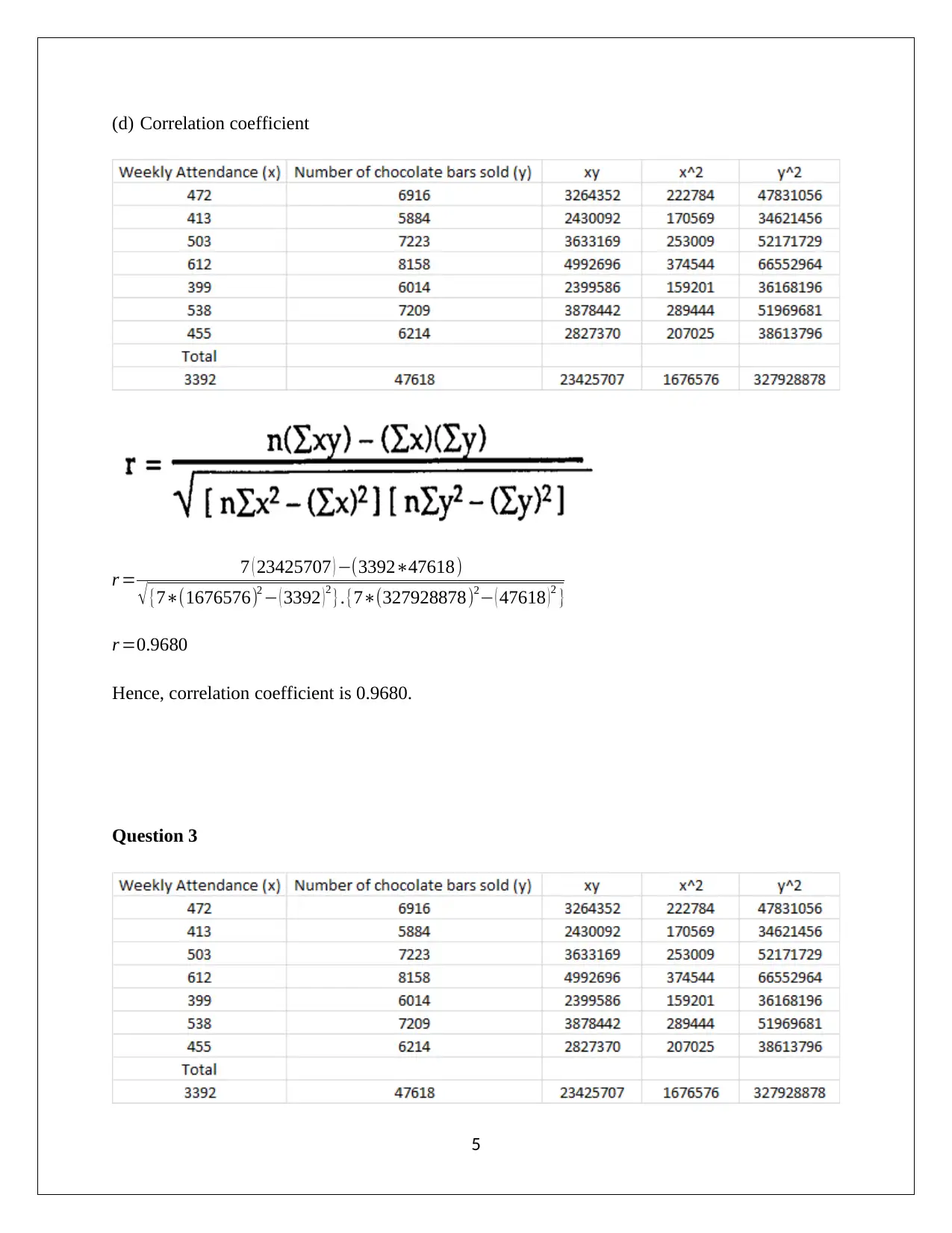
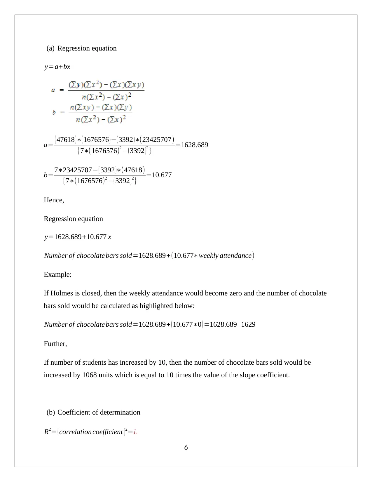
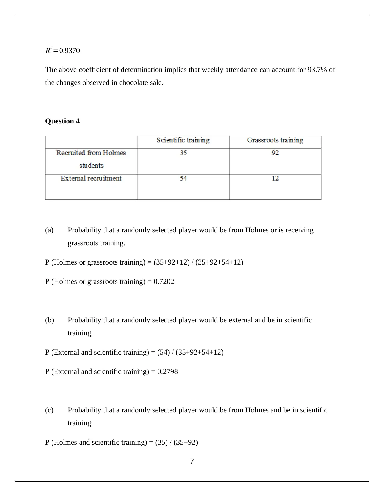
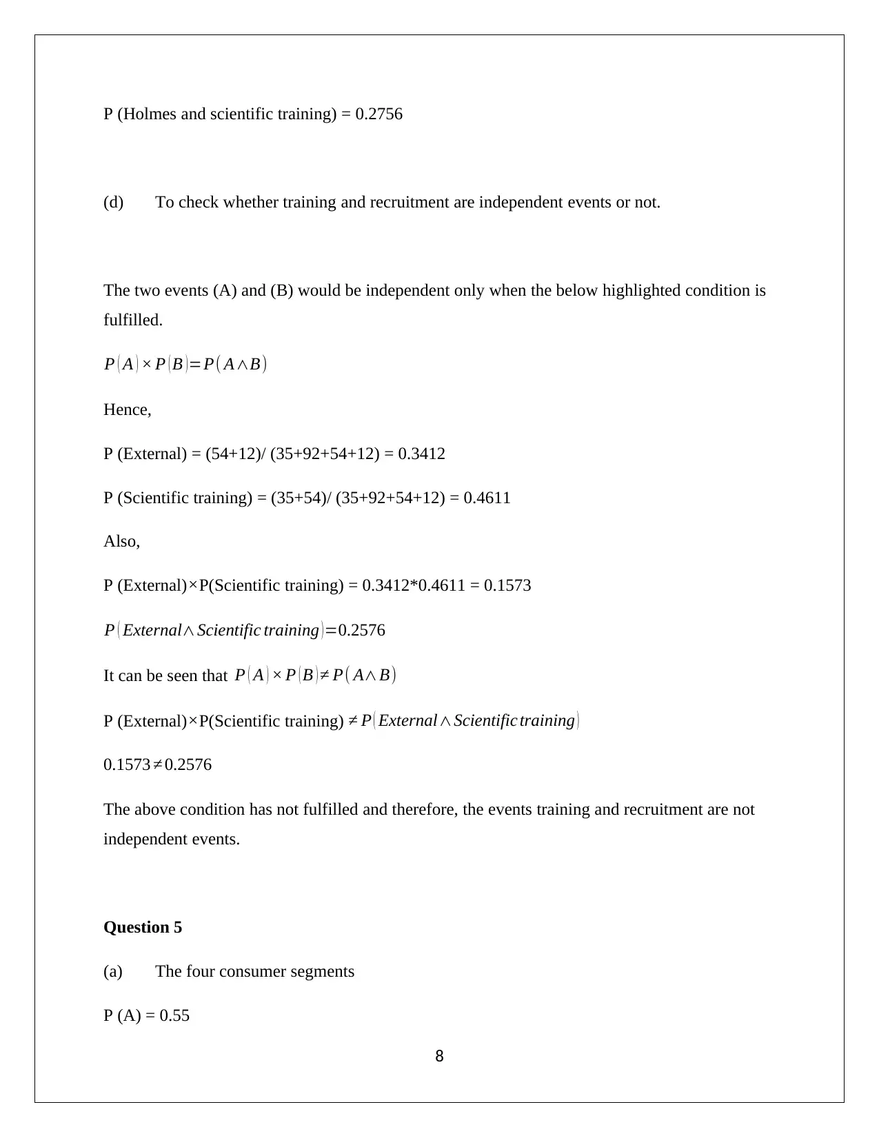
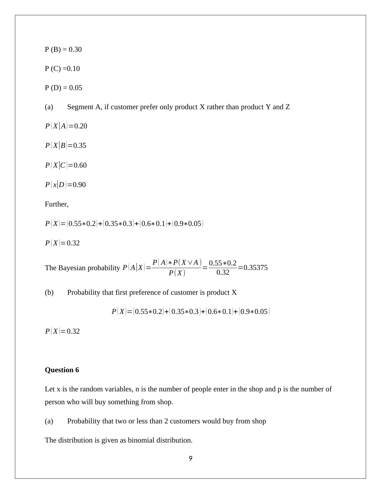
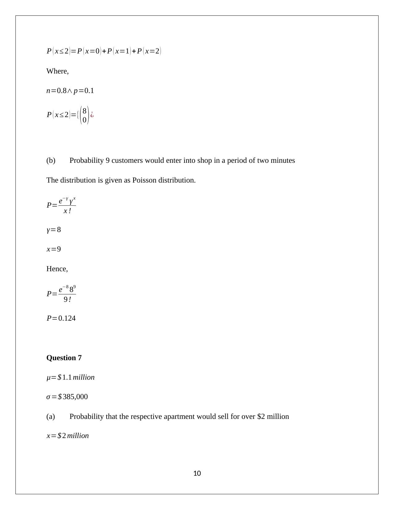
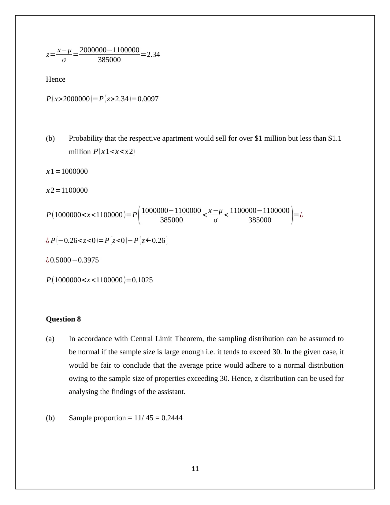
This document provides a detailed solution to an assignment on Applied Quantitative Methods, covering topics such as frequency distribution, histograms, mean, median, mode, standard deviation, interquartile range, correlation coefficient, regression analysis, probability, Bayesian probability, binomial and Poisson distributions, and hypothesis testing. The solution includes calculations and interpretations for various statistical problems, such as analyzing weekly attendance and chocolate bar sales, determining probabilities related to player recruitment and training, and assessing consumer preferences for different products. Furthermore, the assignment applies statistical concepts to real-world scenarios, including property sales and customer behavior, demonstrating the practical application of quantitative methods. Desklib offers a wide range of study resources, including past papers and solved assignments, to support students in their academic endeavors.

APPLIED QUANTITATIVE METHODS
HA1011
Student Name
[Pick the date]

Question 1
(a) Frequency distribution table
(b) Histogram
(c) Mean, median and mode of the data
1

2

The sum of the data = 62006
Total number of observation = 60
Mean = 62006 / 60 =1033.33
It is apparent that the number of observation is an even number and hence, the median would be
calculated shown below:
Median= {( n
2 ) + n+1
2 }
2 = {( 60
2 ) +( 60
2 +1) }
2 = 30 thterm+31thterm
2 = 467+733
2 =715
Maximum frequency from the data comes out for 401 and hence, the mode would be 401.
Question 2
(a) The given data belongs to a sample and not a population. This is apparent from the fact that
the data pertains to only the 7 weeks and does not pertain to the all the weeks when the
university is open. Thus, this data would be termed as sample data and not population data.
(b) Standard deviation of weekly attendance
3

Mean = (472 +413 + 503 + 612 +399 +538 +455) /7 = 484.57
Now,
Standard deviation of sample =
√ ( 32909.7143 )
7−1 =74.06
Therefore, the standard deviation of weekly attendance is 74.06.
(c) Inter quartile range (IQR) for chocolate bars sold
Inter quartile range = Third Quartile – First Quartile
Here,
First Quartile = 25th percentile
ln= ( n+1 )∗P
100 = ( 7+1 )∗25
100 =2 nd term=6014
Third Quartile = 75th percentile
ln= ( n+1 )∗P
100 = ( 7+1 ) ∗75
100 =6 thterm=7223
Thus,
Inter quartile range = Third Quartile – First Quartile
¿ 7223−6014=1209
4

(d) Correlation coefficient
r = 7 ( 23425707 ) −(3392∗47618)
√ {7∗(1676576)2 − ( 3392 ) 2 }.{7∗(327928878)2− ( 47618 ) 2 }
r =0.9680
Hence, correlation coefficient is 0.9680.
Question 3
5

(a) Regression equation
y=a+bx
a= ( 47618 ) ∗( 1676576 ) − ( 3392 ) ∗(23425707)
{7∗( 1676576)2 − ( 3392 ) 2 } =1628.689
b=7∗23425707− ( 3392 )∗(47618)
{7∗(1676576)2 − ( 3392 )2 } =10.677
Hence,
Regression equation
y=1628.689+10.677 x
Number of chocolate bars sold=1628.689+(10.677∗weekly attendance)
Example:
If Holmes is closed, then the weekly attendance would become zero and the number of chocolate
bars sold would be calculated as highlighted below:
Number of chocolate bars sold=1628.689+ ( 10.677∗0 ) =1628.689 1629
Further,
If number of students has increased by 10, then the number of chocolate bars sold would be
increased by 1068 units which is equal to 10 times the value of the slope coefficient.
(b) Coefficient of determination
R2= ( correlation coefficient )2=¿
6

R2=0.9370
The above coefficient of determination implies that weekly attendance can account for 93.7% of
the changes observed in chocolate sale.
Question 4
(a) Probability that a randomly selected player would be from Holmes or is receiving
grassroots training.
P (Holmes or grassroots training) = (35+92+12) / (35+92+54+12)
P (Holmes or grassroots training) = 0.7202
(b) Probability that a randomly selected player would be external and be in scientific
training.
P (External and scientific training) = (54) / (35+92+54+12)
P (External and scientific training) = 0.2798
(c) Probability that a randomly selected player would be from Holmes and be in scientific
training.
P (Holmes and scientific training) = (35) / (35+92)
7

P (Holmes and scientific training) = 0.2756
(d) To check whether training and recruitment are independent events or not.
The two events (A) and (B) would be independent only when the below highlighted condition is
fulfilled.
P ( A ) × P ( B ) =P( A∧B)
Hence,
P (External) = (54+12)/ (35+92+54+12) = 0.3412
P (Scientific training) = (35+54)/ (35+92+54+12) = 0.4611
Also,
P (External) ×P(Scientific training) = 0.3412*0.4611 = 0.1573
P ( External∧Scientific training )=0.2576
It can be seen that P ( A ) × P ( B ) ≠ P( A∧B)
P (External) ×P(Scientific training) ≠ P ( External∧Scientific training )
0.1573 ≠ 0.2576
The above condition has not fulfilled and therefore, the events training and recruitment are not
independent events.
Question 5
(a) The four consumer segments
P (A) = 0.55
8

P (B) = 0.30
P (C) =0.10
P (D) = 0.05
(a) Segment A, if customer prefer only product X rather than product Y and Z
P ( X |A ) =0.20
P ( X |B )=0.35
P ( X |C )=0.60
P ( x|D )=0.90
Further,
P ( X )= ( 0.55∗0.2 ) + ( 0.35∗0.3 )+ ( 0.6∗0.1 )+ ( 0.9∗0.05 )
P ( X )=0.32
The Bayesian probability P ( A |X ) = P ( A )∗P(X ∨A )
P(X ) = 0.55∗0.2
0.32 =0.35375
(b) Probability that first preference of customer is product X
P ( X )= ( 0.55∗0.2 ) + ( 0.35∗0.3 )+ ( 0.6∗0.1 )+ ( 0.9∗0.05 )
P ( X )=0.32
Question 6
Let x is the random variables, n is the number of people enter in the shop and p is the number of
person who will buy something from shop.
(a) Probability that two or less than 2 customers would buy from shop
The distribution is given as binomial distribution.
9

P ( x ≤ 2 )=P ( x=0 ) + P ( x=1 ) + P ( x=2 )
Where,
n=0.8∧ p=0.1
P ( x ≤ 2 ) ={( 8
0 ) ¿
(b) Probability 9 customers would enter into shop in a period of two minutes
The distribution is given as Poisson distribution.
P= e−γ γ x
x !
γ=8
x=9
Hence,
P= e−8 89
9 !
P=0.124
Question 7
μ=$ 1.1 million
σ =$ 385,000
(a) Probability that the respective apartment would sell for over $2 million
x=$ 2 million
10

z= x−μ
σ = 2000000−1100000
385000 =2.34
Hence
P ( x>2000000 ) =P ( z>2.34 ) =0.0097
(b) Probability that the respective apartment would sell for over $1 million but less than $1.1
million P ( x 1< x < x 2 )
x 1=1000000
x 2=1100000
P(1000000< x <1100000)=P ( 1000000−1100000
385000 < x −μ
σ < 1100000−1100000
385000 )=¿
¿ P (−0.26< z <0 )=P ( z <0 )−P ( z←0.26 )
¿ 0.5000−0.3975
P(1000000< x <1100000)=0.1025
Question 8
(a) In accordance with Central Limit Theorem, the sampling distribution can be assumed to
be normal if the sample size is large enough i.e. it tends to exceed 30. In the given case, it
would be fair to conclude that the average price would adhere to a normal distribution
owing to the sample size of properties exceeding 30. Hence, z distribution can be used for
analysing the findings of the assistant.
(b) Sample proportion = 11/ 45 = 0.2444
11

Standard error of sample proportion ¿ √ p (1− p)/n= √ 0.2444 ( 1−0.2444 )
45 =0.064
Further 30% of investors are ready to commit i.e. P ( p >0.30 )
¿ P ( z > 0.3−10.2444
0.064 )
¿ P ( z> 0.87 )
¿ 0.192
12