HA1011 Applied Quantitative Methods Assignment 2 Solution, T1 2019

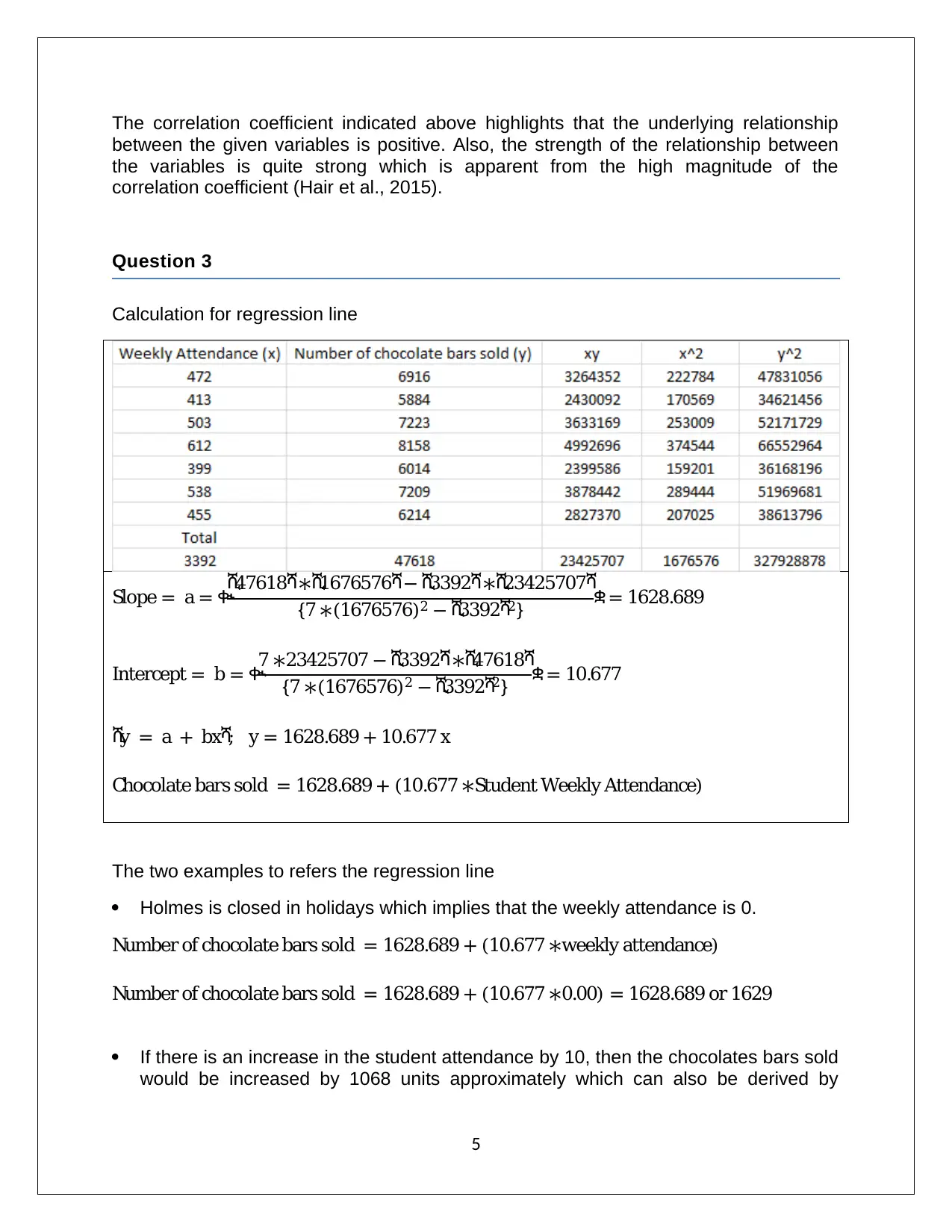
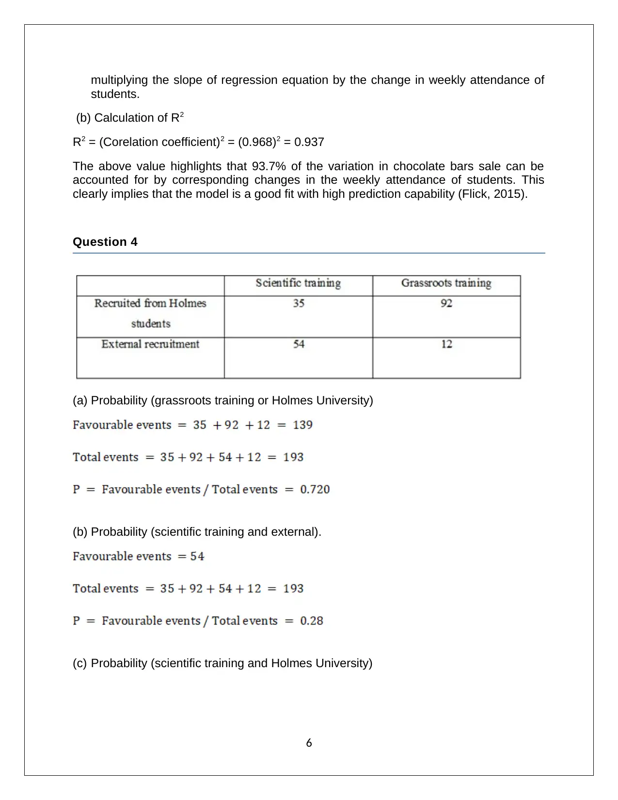
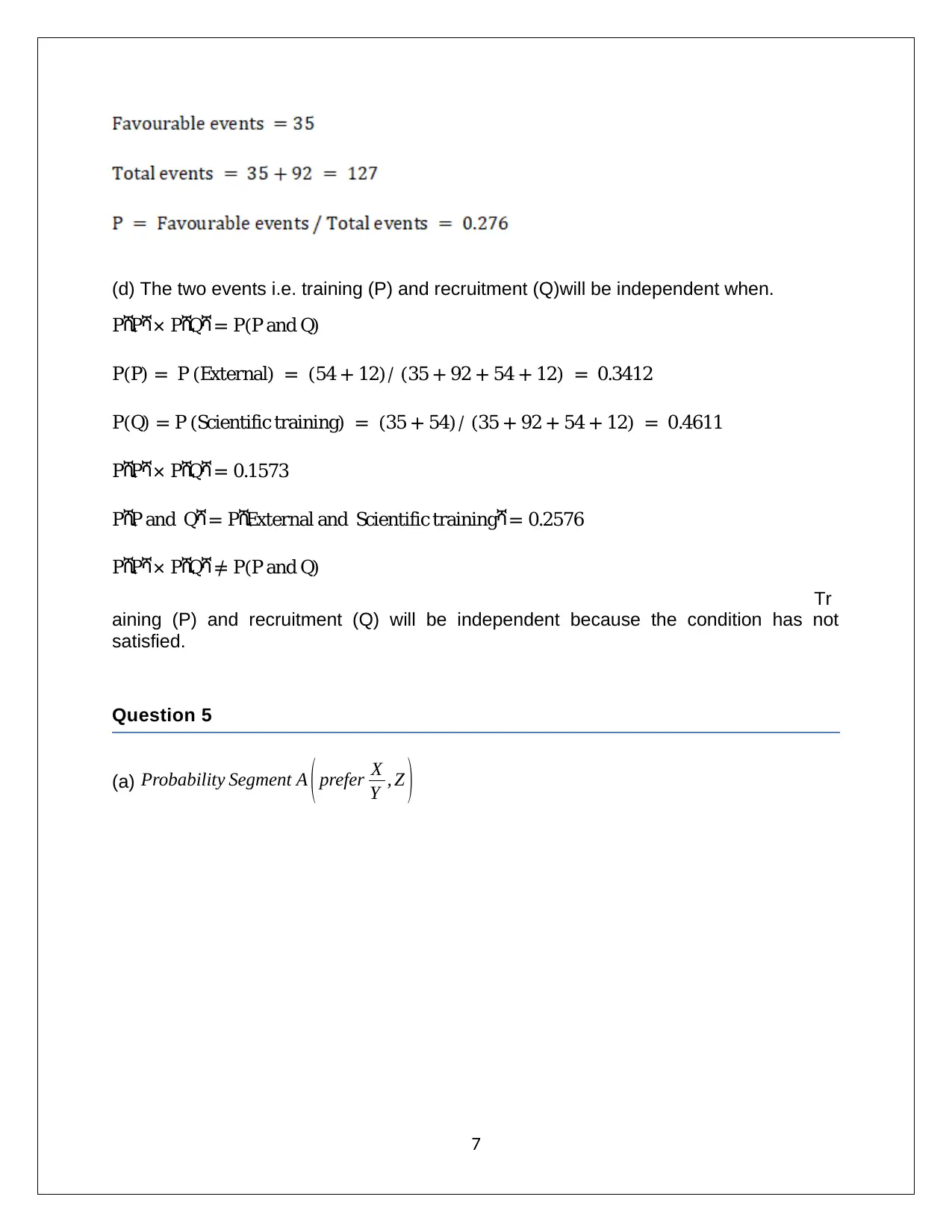
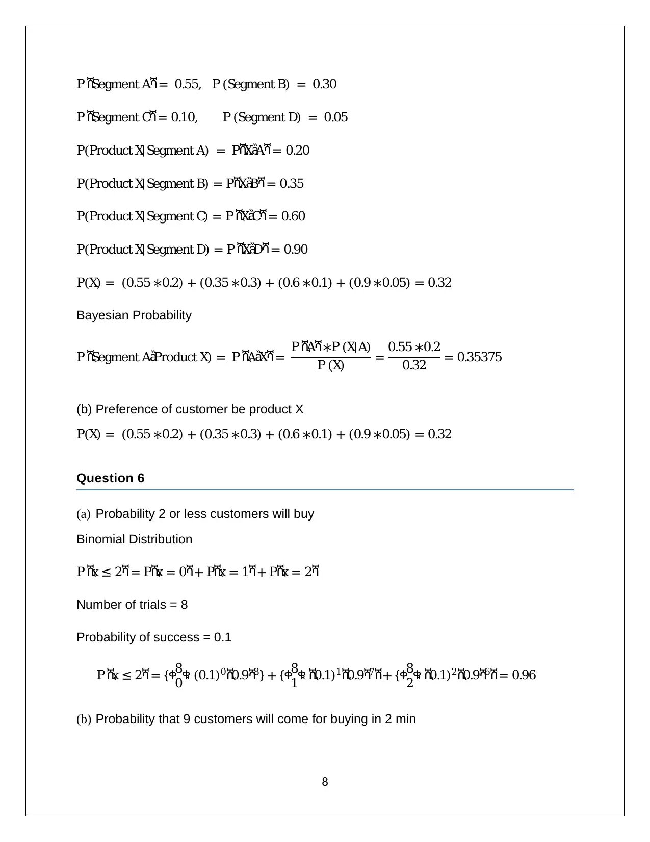
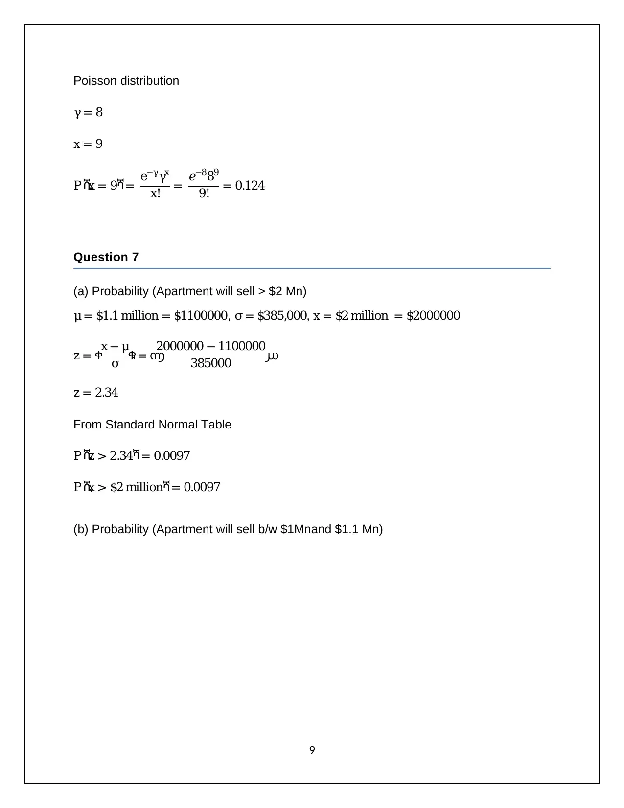
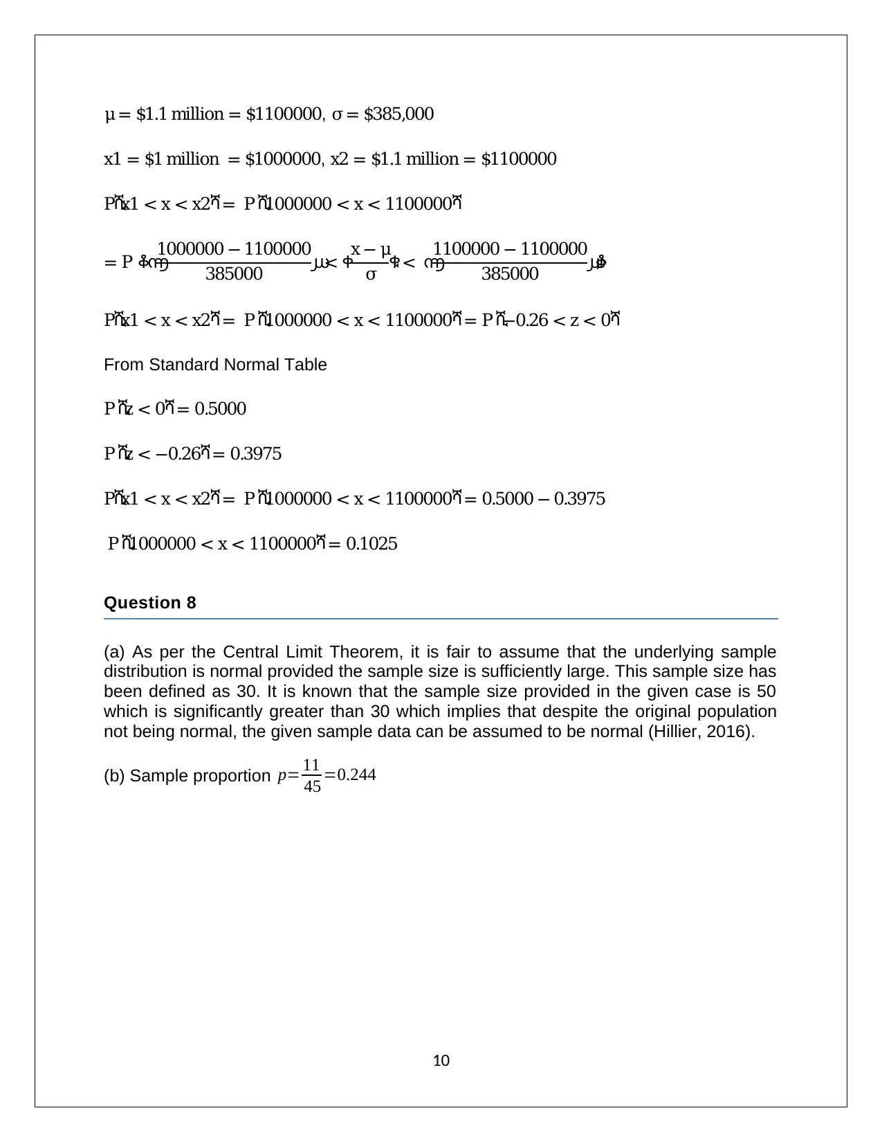
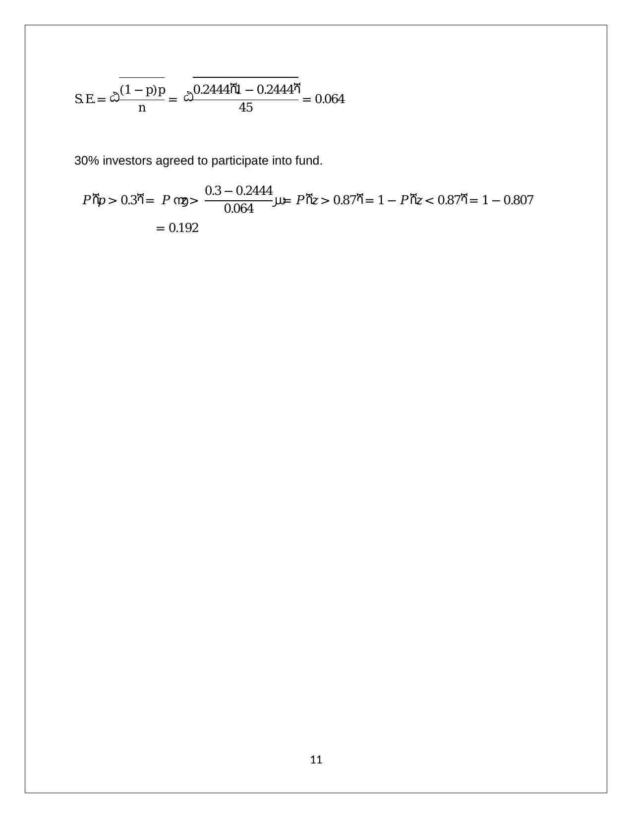
This assignment solution for Applied Quantitative Methods (HA1011) covers a range of statistical concepts and techniques. The solution includes analysis of data, frequency histograms, and measures of central tendency, along with the application of standard deviation, interquartile range, and correlation coefficients. It further delves into regression analysis, calculating the regression line and R-squared values to assess the relationship between variables. The solution also addresses probability calculations involving different scenarios, including Bayesian probability. Additionally, the assignment explores binomial and Poisson distributions, and applies the normal distribution to solve probability problems. Finally, the solution demonstrates the application of the central limit theorem and hypothesis testing to analyze sample data.

APPLIED QUANTITATIVE METHODS
ASSIGNMENT II
Student Name
[Pick the date]

Question 1
(a) Number of passengers at train station (Melbourne)
(b) Frequency histogram
(c) Central tendency measures
1

2

Question 2
(a) The dataset provided is labelled as a sample as it corresponds to selected values
which have been chosen from the population of all weeks in a year. If the given
data corresponded to the population data, then all the 52 weeks contained in a
year would have been represented. Instead only selected values have been
captured which denote a sample.
(b) standard deviation
(c) Inter Quartile Range
3

Sorted
In cases where the underlying data is skewed, standard deviation does not provide an
accurate picture and as a result, it is better to rely on IQR to capture the extent of
dispersion in the data, IQR is not impacted by extreme values (Eriksson and
Kovalainen, 2015).
(d) Correlation coefficient
Correlation coefficient (r) = 0.968
4

The correlation coefficient indicated above highlights that the underlying relationship
between the given variables is positive. Also, the strength of the relationship between
the variables is quite strong which is apparent from the high magnitude of the
correlation coefficient (Hair et al., 2015).
Question 3
Calculation for regression line
Slope = a = ቊ
ሺ47618ሻ∗ሺ1676576ሻ− ሺ3392ሻ∗ሺ23425707ሻ
{7 ∗(1676576)2 − ሺ3392ሻ2} ቋ = 1628.689
Intercept = b = ቊ
7 ∗23425707 − ሺ3392ሻ∗ሺ47618ሻ
{7 ∗(1676576)2 − ሺ3392ሻ2} ቋ = 10.677
ሺy = a + bxሻ; y = 1628.689 + 10.677 x
Chocolate bars sold = 1628.689 + (10.677 ∗Student Weekly Attendance)
The two examples to refers the regression line
 Holmes is closed in holidays which implies that the weekly attendance is 0.
Number of chocolate bars sold = 1628.689 + (10.677 ∗weekly attendance)
Number of chocolate bars sold = 1628.689 + (10.677 ∗0.00) = 1628.689 or 1629
 If there is an increase in the student attendance by 10, then the chocolates bars sold
would be increased by 1068 units approximately which can also be derived by
5

multiplying the slope of regression equation by the change in weekly attendance of
students.
(b) Calculation of R2
R2 = (Corelation coefficient)2 = (0.968)2 = 0.937
The above value highlights that 93.7% of the variation in chocolate bars sale can be
accounted for by corresponding changes in the weekly attendance of students. This
clearly implies that the model is a good fit with high prediction capability (Flick, 2015).
Question 4
(a) Probability (grassroots training or Holmes University)
(b) Probability (scientific training and external).
(c) Probability (scientific training and Holmes University)
6

(d) The two events i.e. training (P) and recruitment (Q)will be independent when.
PሺPሻ× PሺQሻ= P(P and Q)
P(P) = P (External) = (54 + 12)/ (35 + 92 + 54 + 12) = 0.3412
P(Q) = P (Scientific training) = (35 + 54)/ (35 + 92 + 54 + 12) = 0.4611
PሺPሻ× PሺQሻ= 0.1573
PሺP and Qሻ= PሺExternal and Scientific trainingሻ= 0.2576
PሺPሻ× PሺQሻ≠ P(P and Q)
Tr
aining (P) and recruitment (Q) will be independent because the condition has not
satisfied.
Question 5
(a) Probability Segment A ( prefer X
Y , Z )
7

P ሺSegment Aሻ= 0.55, P (Segment B) = 0.30
P ሺSegment Cሻ= 0.10, P (Segment D) = 0.05
P(Product X|Segment A) = PሺXa=Aሻ= 0.20
P(Product X|Segment B) = PሺXa=Bሻ= 0.35
P(Product X|Segment C) = P ሺXa=Cሻ= 0.60
P(Product X|Segment D) = P ሺXa=Dሻ= 0.90
P(X) = (0.55 ∗0.2) + (0.35 ∗0.3) + (0.6 ∗0.1) + (0.9 ∗0.05) = 0.32
Bayesian Probability
P ሺSegment Aa=Product X) = P ሺAa=Xሻ= P ሺAሻ∗P (X|A)
P (X) = 0.55 ∗0.2
0.32 = 0.35375
(b) Preference of customer be product X
P(X) = (0.55 ∗0.2) + (0.35 ∗0.3) + (0.6 ∗0.1) + (0.9 ∗0.05) = 0.32
Question 6
(a) Probability 2 or less customers will buy
Binomial Distribution
P ሺx ≤ 2ሻ= Pሺx = 0ሻ+ Pሺx = 1ሻ+ Pሺx = 2ሻ
Number of trials = 8
Probability of success = 0.1
P ሺx ≤ 2ሻ= {ቀ8
0ቁ (0.1)0ሺ0.9ሻ8} + {ቀ8
1ቁ ሺ0.1)1ሺ0.9ሻ7ሽ+ {ቀ8
2ቁ ሺ0.1)2ሺ0.9ሻ6ሽ= 0.96
(b) Probability that 9 customers will come for buying in 2 min
8

Poisson distribution
γ = 8
x = 9
P ሺx = 9ሻ= e−γγx
x! = 𝑒−889
9! = 0.124
Question 7
(a) Probability (Apartment will sell > $2 Mn)
μ= $1.1 million = $1100000, σ= $385,000, x = $2 million = $2000000
z = ቀx − μ
σ ቁ = ൬
2000000 − 1100000
385000 ൰
z = 2.34
From Standard Normal Table
P ሺz > 2.34ሻ= 0.0097
P ሺx > $2 millionሻ= 0.0097
(b) Probability (Apartment will sell b/w $1Mnand $1.1 Mn)
9

μ= $1.1 million = $1100000, σ= $385,000
x1 = $1 million = $1000000, x2 = $1.1 million = $1100000
Pሺx1 < x < x2ሻ= P ሺ1000000 < x < 1100000ሻ
= P ቆ൬
1000000 − 1100000
385000 ൰< ቀx − μ
σ ቁ < ൬
1100000 − 1100000
385000 ൰ቇ
Pሺx1 < x < x2ሻ= P ሺ1000000 < x < 1100000ሻ= P ሺ−0.26 < z < 0ሻ
From Standard Normal Table
P ሺz < 0ሻ= 0.5000
P ሺz < −0.26ሻ= 0.3975
Pሺx1 < x < x2ሻ= P ሺ1000000 < x < 1100000ሻ= 0.5000 − 0.3975
P ሺ1000000 < x < 1100000ሻ= 0.1025
Question 8
(a) As per the Central Limit Theorem, it is fair to assume that the underlying sample
distribution is normal provided the sample size is sufficiently large. This sample size has
been defined as 30. It is known that the sample size provided in the given case is 50
which is significantly greater than 30 which implies that despite the original population
not being normal, the given sample data can be assumed to be normal (Hillier, 2016).
(b) Sample proportion p= 11
45 =0.244
10

30% investors agreed to participate into fund.
𝑃ሺ𝑝 > 0.3ሻ= 𝑃 ൬𝑧> 0.3 − 0.2444
0.064 ൰= 𝑃ሺ𝑧> 0.87ሻ= 1 − 𝑃ሺ𝑧< 0.87ሻ= 1 − 0.807
= 0.192
S.E.= ඨ(1 − p)p
n = ඨ0.2444ሺ1 − 0.2444ሻ
45 = 0.064
11

References
Eriksson, P. and Kovalainen, A. (2015) Quantitative methods in business research. 3rd
ed. London: Sage Publications, pp. 115
Flick, U. (2015) Introducing research methodology: A beginner's guide to doing a
research project. 4th ed. New York: Sage Publications, pp. 206
Hair, J. F., Wolfinbarger, M., Money, A. H., Samouel, P., and Page, M. J.
(2015) Essentials of business research methods. 2nd ed. New York: Routledge, pp. 165
Hillier, F. (2016) Introduction to Operations Research.6th ed.New York: McGraw Hill
Publications, pp. 189
12