Applied Managerial Statistics - Sales Prediction: Maths 534 Report

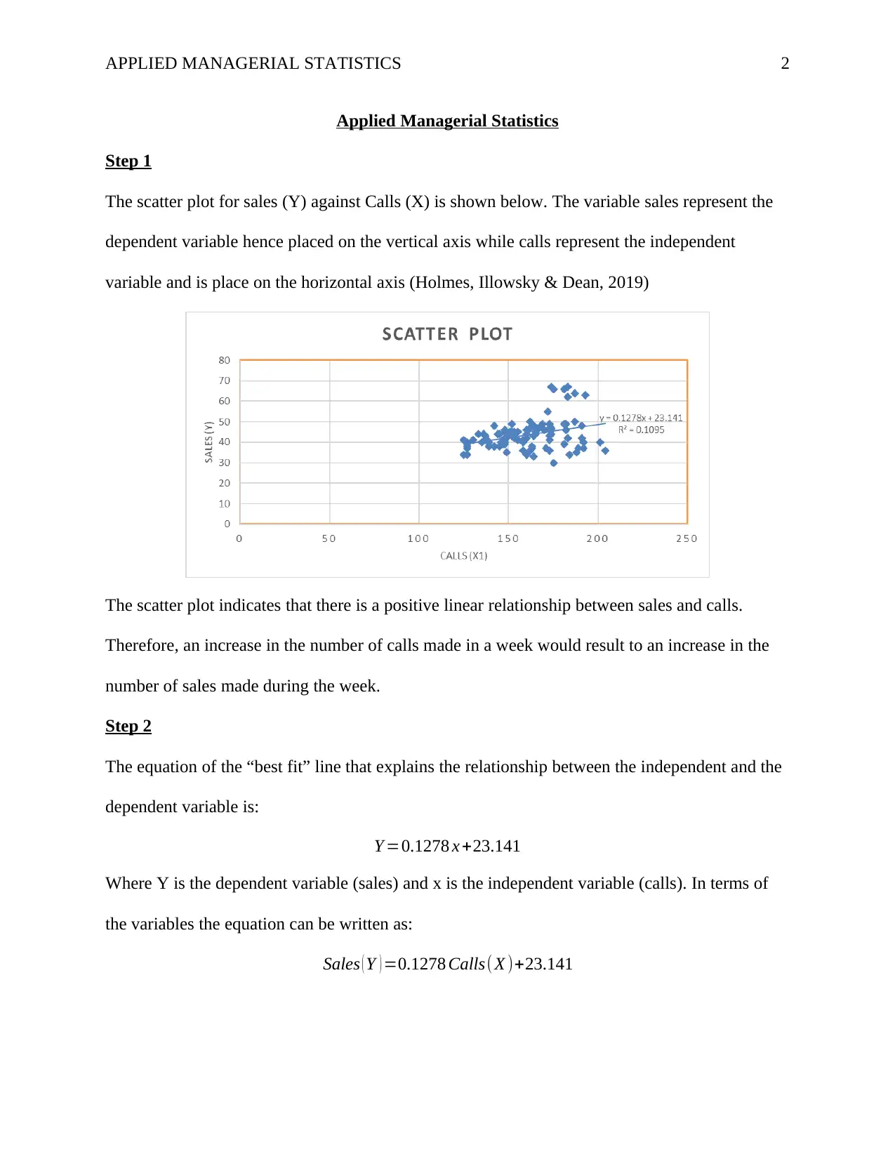
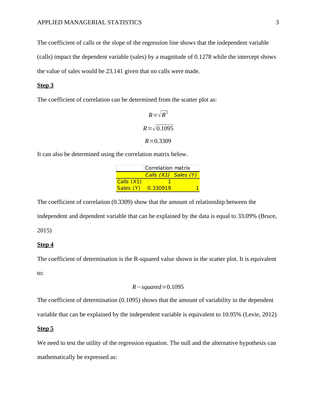
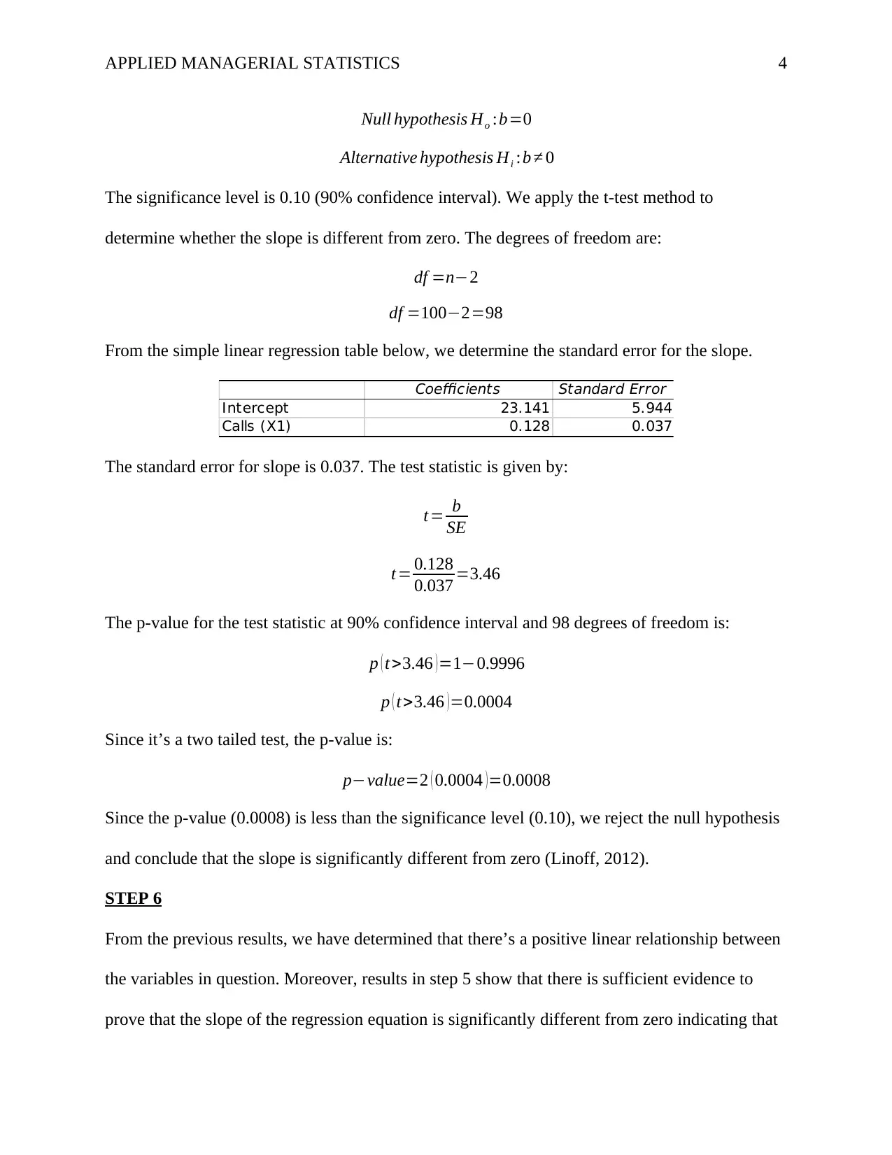
This report presents a comprehensive analysis of sales data using applied managerial statistics. It begins with a scatter plot illustrating the relationship between sales and calls, followed by the derivation of a regression equation to model this relationship. The report then calculates the coefficient of correlation and determination to quantify the strength of the relationship. Hypothesis testing is conducted to assess the utility of the regression equation, and confidence intervals are computed for the slope and predicted values. The analysis culminates in the determination of prediction intervals and a discussion of the implications for business decision-making, particularly regarding the optimal number of sales calls to maximize sales. The report utilizes statistical methods to provide insights into sales trends and offers data-driven recommendations for business strategy.

Running head: APPLIED MANAGERIAL STATISTICS 1
Maths 534: Applied Managerial Statistics
Student Name
Professor’s Name
University Name
Date

APPLIED MANAGERIAL STATISTICS 2
Applied Managerial Statistics
Step 1
The scatter plot for sales (Y) against Calls (X) is shown below. The variable sales represent the
dependent variable hence placed on the vertical axis while calls represent the independent
variable and is place on the horizontal axis (Holmes, Illowsky & Dean, 2019)
The scatter plot indicates that there is a positive linear relationship between sales and calls.
Therefore, an increase in the number of calls made in a week would result to an increase in the
number of sales made during the week.
Step 2
The equation of the “best fit” line that explains the relationship between the independent and the
dependent variable is:
Y =0.1278 x +23.141
Where Y is the dependent variable (sales) and x is the independent variable (calls). In terms of
the variables the equation can be written as:
Sales ( Y ) =0.1278 Calls( X )+23.141

APPLIED MANAGERIAL STATISTICS 3
The coefficient of calls or the slope of the regression line shows that the independent variable
(calls) impact the dependent variable (sales) by a magnitude of 0.1278 while the intercept shows
the value of sales would be 23.141 given that no calls were made.
Step 3
The coefficient of correlation can be determined from the scatter plot as:
R= √ R2
R= √ 0.1095
R=0.3309
It can also be determined using the correlation matrix below.
Correlation matrix
Calls (X1) Sales (Y)
Calls (X1) 1
Sales (Y) 0.330919 1
The coefficient of correlation (0.3309) show that the amount of relationship between the
independent and dependent variable that can be explained by the data is equal to 33.09% (Bruce,
2015)
Step 4
The coefficient of determination is the R-squared value shown in the scatter plot. It is equivalent
to:
R−squared=0.1095
The coefficient of determination (0.1095) shows that the amount of variability in the dependent
variable that can be explained by the independent variable is equivalent to 10.95% (Levie, 2012)
Step 5
We need to test the utility of the regression equation. The null and the alternative hypothesis can
mathematically be expressed as:

APPLIED MANAGERIAL STATISTICS 4
Null hypothesis Ho :b=0
Alternative hypothesis Hi :b ≠ 0
The significance level is 0.10 (90% confidence interval). We apply the t-test method to
determine whether the slope is different from zero. The degrees of freedom are:
df =n−2
df =100−2=98
From the simple linear regression table below, we determine the standard error for the slope.
Coefficients Standard Error t Stat P-value
Intercept 23.141 5.944 3.893 0.000
Calls (X1) 0.128 0.037 3.472 0.001
The standard error for slope is 0.037. The test statistic is given by:
t= b
SE
t= 0.128
0.037 =3.46
The p-value for the test statistic at 90% confidence interval and 98 degrees of freedom is:
p ( t>3.46 ) =1−0.9996
p ( t>3.46 )=0.0004
Since it’s a two tailed test, the p-value is:
p−value=2 ( 0.0004 )=0.0008
Since the p-value (0.0008) is less than the significance level (0.10), we reject the null hypothesis
and conclude that the slope is significantly different from zero (Linoff, 2012).
STEP 6
From the previous results, we have determined that there’s a positive linear relationship between
the variables in question. Moreover, results in step 5 show that there is sufficient evidence to
prove that the slope of the regression equation is significantly different from zero indicating that

APPLIED MANAGERIAL STATISTICS 5
there is a statistically significant relationship between sales and calls. Therefore, we can
conclude that the independent variable can conveniently predict the dependent variable.
Step 7
We need to determine the 95% confidence interval of the slope. The slope is 0.128. The alpha
value for 95% confidence interval is:
∝=1− CL
100
∝=1− 95
100
∝=0.05
The critical probability for the confidence interval is:
P¿=1− ∝
2
P¿=1− 0.05
2 =0.975
The degrees of freedom are:
df =n−2
df =100−2=98
The critical value for 98 df and 0.975 critical probability is 1.984. The margin of error is given
by:
ME=critical value∗standard error
ME=1.984∗0.037=0.0734
The confidence interval lower and upper limit is:
Lower limit =0.128−0.0734=0.0546
upper limit=0.128+0.0734=0.2014
The confidence interval for the slope is:

APPLIED MANAGERIAL STATISTICS 6
CI =0.0546 ≤ b ≤0.2014
The confidence interval means that there is a 95% guarantee that the true slope of the regression
equation9of the variables falls between 0.0546 and 0.2014 (Lock, 2013).
Step 8
We are to determine the 99% confidence interval of the dependent variable for any given value
of the independent variable. The selected value of the independent variable is 150 calls. The
regression equation is:
Sales ( Y ) =0.1278 Calls( X )+23.141
Substituting the selected value, we have:
Sales ( Y ) =0.1278(150)+23.141
Sales ( Y ) =42.311
We use the ANOVA table shown below to simplify the computations.
ANOVA
df SS MS F Significance F
Regression 1 600.025 600.025 12.051 0.001
Residual 98 4879.285 49.789
Total 99 5479.310
The standard error of the estimate from the table is:
SSerror =4879.285
The mean squared error is given by:
MSE= SSerror
n−2
MSE= 4879.285
98 =49.79
The standard error of estimate is therefore:
^σ = √ MSE
^σ = √49.79=7.056

APPLIED MANAGERIAL STATISTICS 7
Sum of squares are given by:
SSxx=∑
i=1
n
x2− 1
n (∑
i=1
n
x )2
SSxx=2607311− 1
100 ( 16033 )2
SSxx=36740.11
SSyy =∑
i=1
n
y2− 1
n ( ∑
i=1
n
y )
2
SSyy =195837− 1
100 ( 4363 )2
SSyy =5479.31
The significance level is 0.01 and the degrees of freedom are 98 as computed previously. The
critical value of t for these values is 2.627. The margin of error is given by:
ME=tc √ ^σ2 ¿ ¿
ME=2.627 √49.79 ¿ ¿
ME=2.106
The 99% confidence interval for the predicted value is:
Lower limit =42.311−2.106=40.205
upper limit=42.311+2.106=44.417
CI =40.205 ≤ Y ≤ 44.417
The confidence interval means that there is 99% guarantee that the predicted value of sales will
be between 40.205 and 44.417 (Croucher, 2016).
Step 9
We are to determine the 99% prediction interval using values selected in the previous question.
The formula for margin of error for the prediction interval is:

APPLIED MANAGERIAL STATISTICS 8
ME=tc √ ^σ2 ¿ ¿
ME=2.627 √49.79 ¿ ¿
ME=18.656
The prediction interval is:
Lower limit =42.311−18.656=23.655
upper limit=42.311+18.656=60.967
PI =23.655 ≤Y ≤ 60.967
The prediction interval means that there is a 99% guarantee that future predicted value of sales
will fall between the range of 23.655 and 60.967
Step 10
When the values of independent variable that are outside the range of the sample values, we can
say that the values of the dependent variable will not be entirely accurate and hence not reliable
for prediction. This is because the model is created to predict the dependent variable using values
of the independent variable that fall within the sample. If an accepted statistical margin of
variation is surpassed, the prediction will not be accurate hence unreliable.
Step 11
The business decision that can be made based on the result of this analysis is determination of
the number of calls that should be made in a week to maximize sales. Since the sales increase
with number of calls made in a week, the management can decide to settle on a minimum
threshold number of calls that should be made in a week to maximize the sales. Through
determination of the number of sales that should be made to maximize sales, business operation
may change by ensuring that more customers are contacted and the conversion rate of customers
called to sales for the business would increase resulting to more profit for the entity.

APPLIED MANAGERIAL STATISTICS 9

APPLIED MANAGERIAL STATISTICS 10
References
Bruce, P. (2015). Introductory statistics and analytics. New Jersey: Wiley.
Croucher, J. S. (2016). Introductory mathematics & statistics.6th ed. Australia: North Ryde,
N.S.W. McGraw-Hill Education.
Levie, R. D. (2012). Advanced Excel for scientific data analysis (2nd ed). New York, NY: Oxford
University Press.
Linoff, G. (2012). Data analysis using SQL and Excel. Indianapolis, Ind.: Wiley Pub.
Lock, R. (2013). Statistics: Unlocking the power of data. Wiley.
Holmes, A., Illowsky, B., & Dean, S. (2019). Introductory business statistics. OpenStax.