Applied Econometrics: ARDL Model for Australian All Ordinaries Index

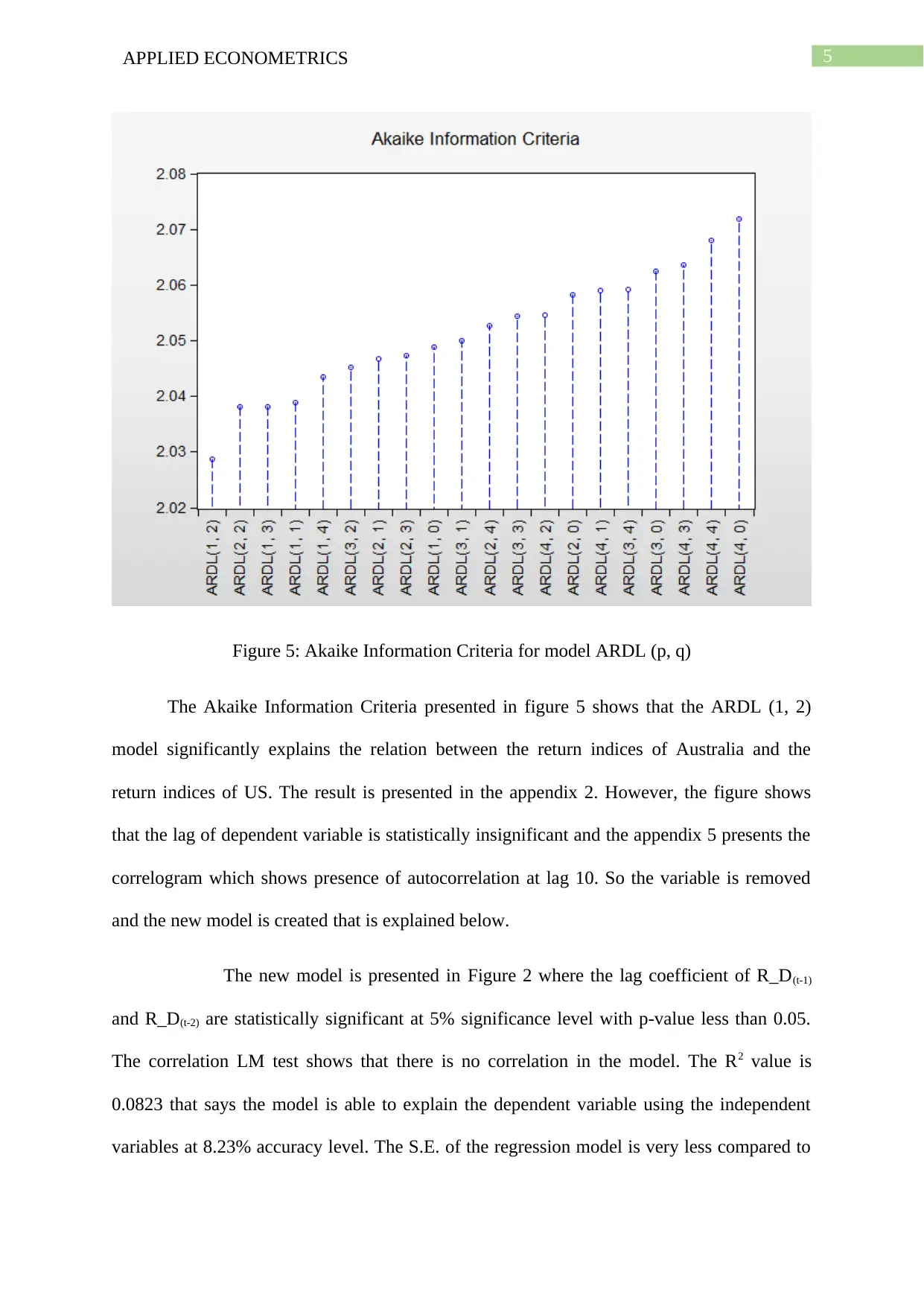
This assignment presents an econometric analysis of the Australian All Ordinaries Index using an Autoregressive Distributed Lag (ARDL) model. It investigates the influence of foreign market indices, particularly the US Dow Jones and the Hong Kong Hang Seng, on Australian returns. The report details the process of selecting appropriate lag structures to ensure goodness of fit and eliminate autocorrelation, presenting the estimated equation and supporting outputs. It discusses the dynamics of returns, identifies key foreign influences, and assesses the model's fit, highlighting implications for financial modeling. Additionally, the assignment includes an analysis of infant mortality rates using multivariate linear regression, exploring the impact of factors like contraceptive use, GDP, sanitation, and education. The strengths and weaknesses of the model are discussed, along with its predictive capabilities.

Running head: APPLIED ECONOMETRICS
Applied Econometrics
Name of the Student:
Name of the University:
Author Note:

1APPLIED ECONOMETRICS
Table of Contents
Answer Q3.................................................................................................................................2
Answer 1................................................................................................................................2
Answer 2................................................................................................................................4
Answer 3................................................................................................................................6
Answer Q3.................................................................................................................................6
Reference and Bibliography.......................................................................................................9
Appendices...............................................................................................................................10

2APPLIED ECONOMETRICS
Answer Q3
Answer 1
The figure presents the residuals correlogram which shows that there is no
autocorrelation within the data.
Figure 1: Residual Correlogram
Moreover, the Breusch-Godfrey Serial Correlation LM test states about the
correlation within the model ARLD (0, 2). The null hypothesis and the alternative hypothesis
of the LM test is mentioned below:
H0: p = 0
H1: p ≠ 0

3APPLIED ECONOMETRICS
Figure 2: LM test to check the presence of autocorrelation
The p-value is 0.4961 which is greater than 0.05. This indicates that there is not
enough evidence to reject the null hypothesis and thus the null hypothesis is accepted and the
model is free from autocorrelation (Brooks 2019).
Figure 3: EViews ARDL (0, 2) Outtput
The ARLD (0, 2) model is presented below:
R_A = B1 R_Dt + B2 R_D (t-1) + B3 R_D (t-2)
The estimated model based on the results from the figure 3 where the result is
presented, is as follows:
R_A = (0.1820 * R_Dt) + (0.0956 * R_D (t-1)) - (0.1018 * R_D (t-2))
This model reduced the autocorrelation and can better explain the daily return through
the indices (Gourieroux and Jasiak 2018). The model incorporate 2 independent lag variables

4APPLIED ECONOMETRICS
of return index of US. Moreover, based on the correlation LM test, autocorrelation does not
exist in the data set.
Answer 2
Figure 4: Akaike Information Criteria for model ARDL (p, q1, q2)
The Akaike Information Criteria presented in figure 4 shows that the ARDL (1, 2, 0)
model significantly explains the relation between the return indices of Australia and the
return indices of US and Hong Kong. The result is presented in the appendix 3. However, the
figure shows that the lag of dependent variable and the return index of Hong Kong are
statistically insignificant and the appendix 3 shows that there exists an autocorrelation at lag
10 (Asteriou and Hall 2015). So the variables are removed and the new model is created that
are explained below:

5APPLIED ECONOMETRICS
Figure 5: Akaike Information Criteria for model ARDL (p, q)
The Akaike Information Criteria presented in figure 5 shows that the ARDL (1, 2)
model significantly explains the relation between the return indices of Australia and the
return indices of US. The result is presented in the appendix 2. However, the figure shows
that the lag of dependent variable is statistically insignificant and the appendix 5 presents the
correlogram which shows presence of autocorrelation at lag 10. So the variable is removed
and the new model is created that is explained below.
The new model is presented in Figure 2 where the lag coefficient of R_D(t-1)
and R_D(t-2) are statistically significant at 5% significance level with p-value less than 0.05.
The correlation LM test shows that there is no correlation in the model. The R2 value is
0.0823 that says the model is able to explain the dependent variable using the independent
variables at 8.23% accuracy level. The S.E. of the regression model is very less compared to

6APPLIED ECONOMETRICS
the sample size of the model that indicates the variation of the overall prediction or the
estimation.
Answer 3
On the basis of the model ARDL (0, 2), return index of Australia is significantly
dependent on the return index of US and the 2 lags of these variable. The regression
coefficient is 0.0823 and the overall SE is 0.6564. The independent variables are statistically
significant within the 95% confidence interval. Due to one unit change in the return index of
US can raise the return index of Australia by 0.182 units considering there is no lag period.
This suggest there is significant influence on the return index of Australia.
The return index of US is more important for the returns in Australia as the variable in
the model is significant and the return index of Hong Kong is not significant. It takes two
years to US return index to reduce the return index of Australia by -0.1018%. This means that
the current index of Australia is influenced negatively by the growth of return index in US.
Answer Q3
The model is presented below:
infant mortality=β0 + β1 contraceptive+ β2 GDP+ β3 sanitation+ β4 education∗contraceptive+ β5 education∗ph
The estimated model is presented below:
i nfant mortality =105.71−1.30 4∗c ontraceptive−0.0003∗GDP−0.007∗sanitation+0.0886∗education∗con

7APPLIED ECONOMETRICS
Figure 6: Regression Result
The adjusted R2 for the above multivariate linear regression model is 0.7769 which
explains the 77.69% of the variance accurately and the p-value of the F-statistics is 0.00
which indicates that the model is best explained with the help of the incorporated independent
variables (Wooldridge 2015). All the mentioned variables in the above table are statistically
significant have a influence on the infant mortality. The initial model presented in the
appendix 6 shows that the education variable is insignificant then the variable is dropped and
incorporated as the interaction variable as the adjusted R2 value was reduced due to omitting
the insignificant variables and the process is repeated for insignificant variables and finally
the above model is constructed.
The F-statistics of the model is significant and the incorporated independent variables
are significant at 5% significance level. Hence, the model is appropriate for the data.

8APPLIED ECONOMETRICS
The strengths of the model is that it incorporates the interaction variable education
while it was insignificant but had an impact on the infant mortality. The problem is solved by
the interaction of education with the other variables. The weakness of the model is that it
cannot explain the time and place though the data provides the information about these
variables.
The linear model is easy to explain and also easy to perform and interpret the results.
The model can be used to predict the infant mortality with the given information. The
observation is quite large and the standard error is low comparatively, implies the variation is
less in the prediction. The large data with minimum errors indicates the small value of SE.
There is no multicollinearity in the model as there does not exist any similar type of
independent variable. The infant mortality can be predicted easily by the above mentioned
variables in the regression result table.

9APPLIED ECONOMETRICS
Reference and Bibliography
Aljandali, A. and Tatahi, M., 2018. Economic and Financial Modelling with EViews: A
Guide for Students and Professionals. Springer.
Asteriou, D. and Hall, S.G., 2015. Applied econometrics. Macmillan International Higher
Education.
Brooks, C., 2019. Introductory econometrics for finance. Cambridge university press.
Gourieroux, C. and Jasiak, J., 2018. Financial econometrics: Problems, models, and methods.
Princeton University Press.
Hendrych, R. and Cipra, T., 2017. Econometric model of non-life technical provisions: the
Czech insurance market case study. European Actuarial Journal, 7(1), pp.257-276.
Ma, L., Hu, C., Lin, R. and Han, Y., 2018, December. ARIMA model forecast based on
EViews software. In IOP Conference Series: Earth and Environmental Science (Vol. 208,
No. 1, p. 012017). IOP Publishing.
Rădulescu, C. and Hudea, O.S., 2018. Econometric modelling of the consumer’s behaviour in
order to develop brand management policies. Economic research-Ekonomska
istraživanja, 31(1), pp.576-591.
Wooldridge, J.M., 2015. Introductory econometrics: A modern approach. Nelson Education.

10APPLIED ECONOMETRICS
Appendices
Appendix 1: Table of residuals in ARLD (0, 2) model
Appendix 2: The ALRD (1, 2, 0) model

11APPLIED ECONOMETRICS
Appendix 3: The residuals correlogram for ALRD (1, 2, 0) model
Appendix 4: The ALRD (1, 2) model
Appendix 5: The residuals correlogram for ALRD (1, 2) model

12APPLIED ECONOMETRICS
Appendix 6: Regression result of initial model

13APPLIED ECONOMETRICS