Comprehensive Report: 3-Band Audio Amplifier Design and Analysis

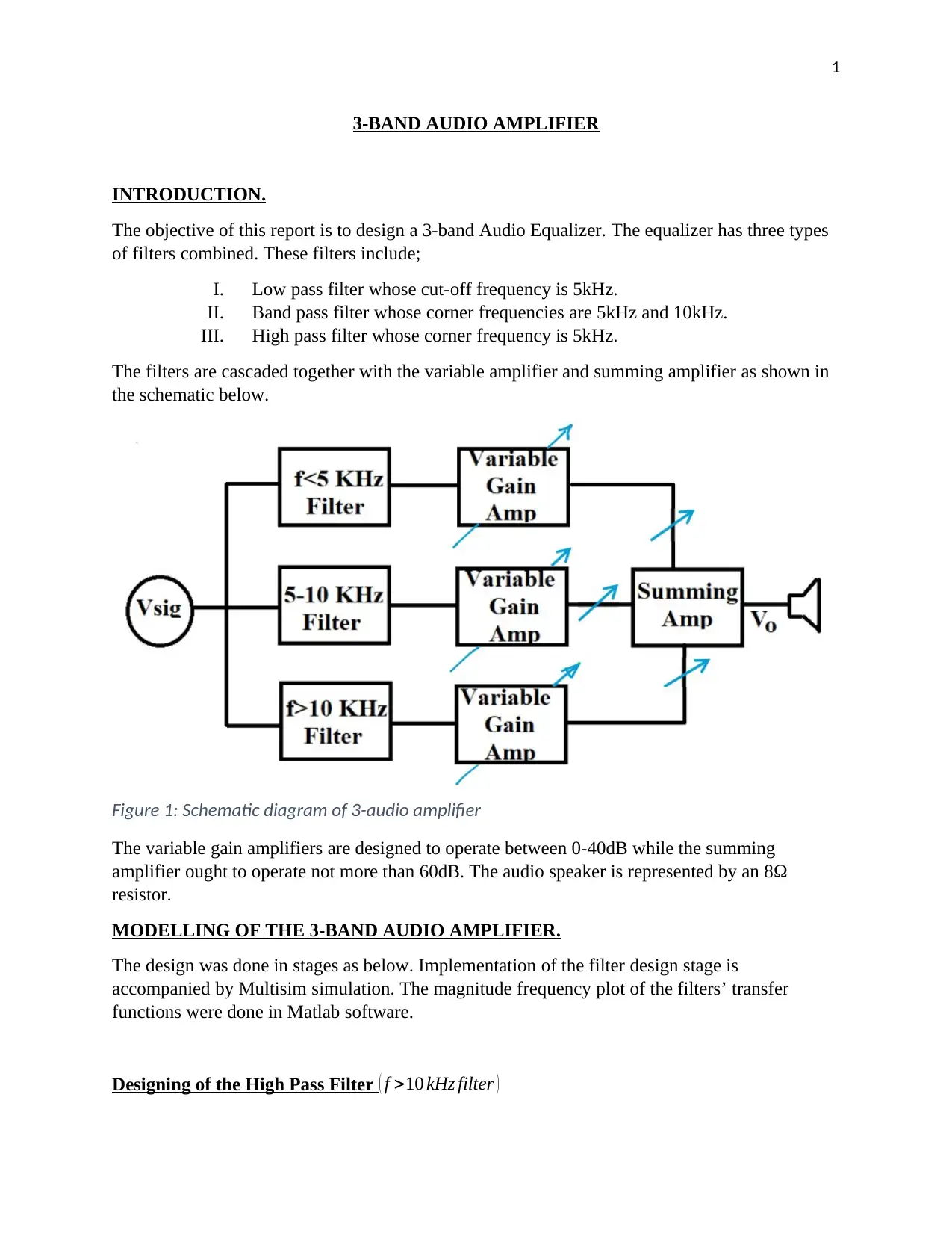
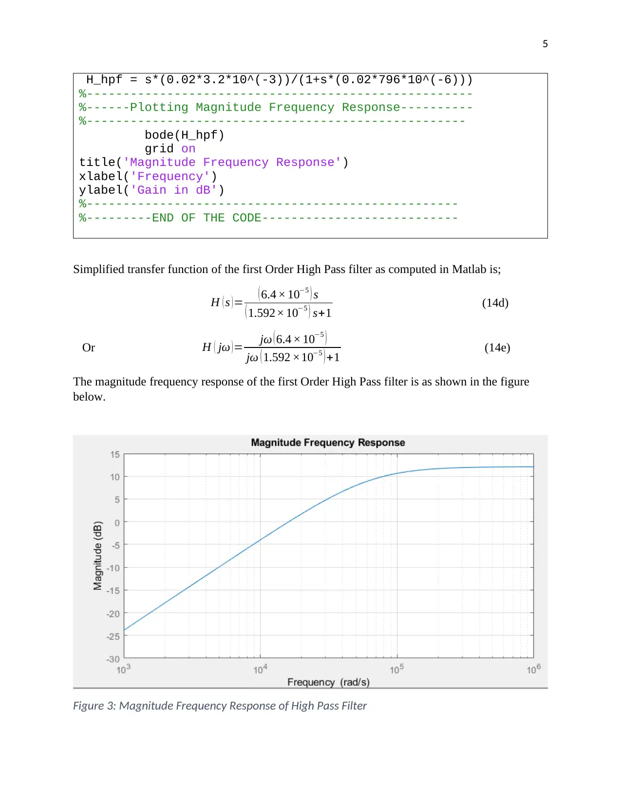
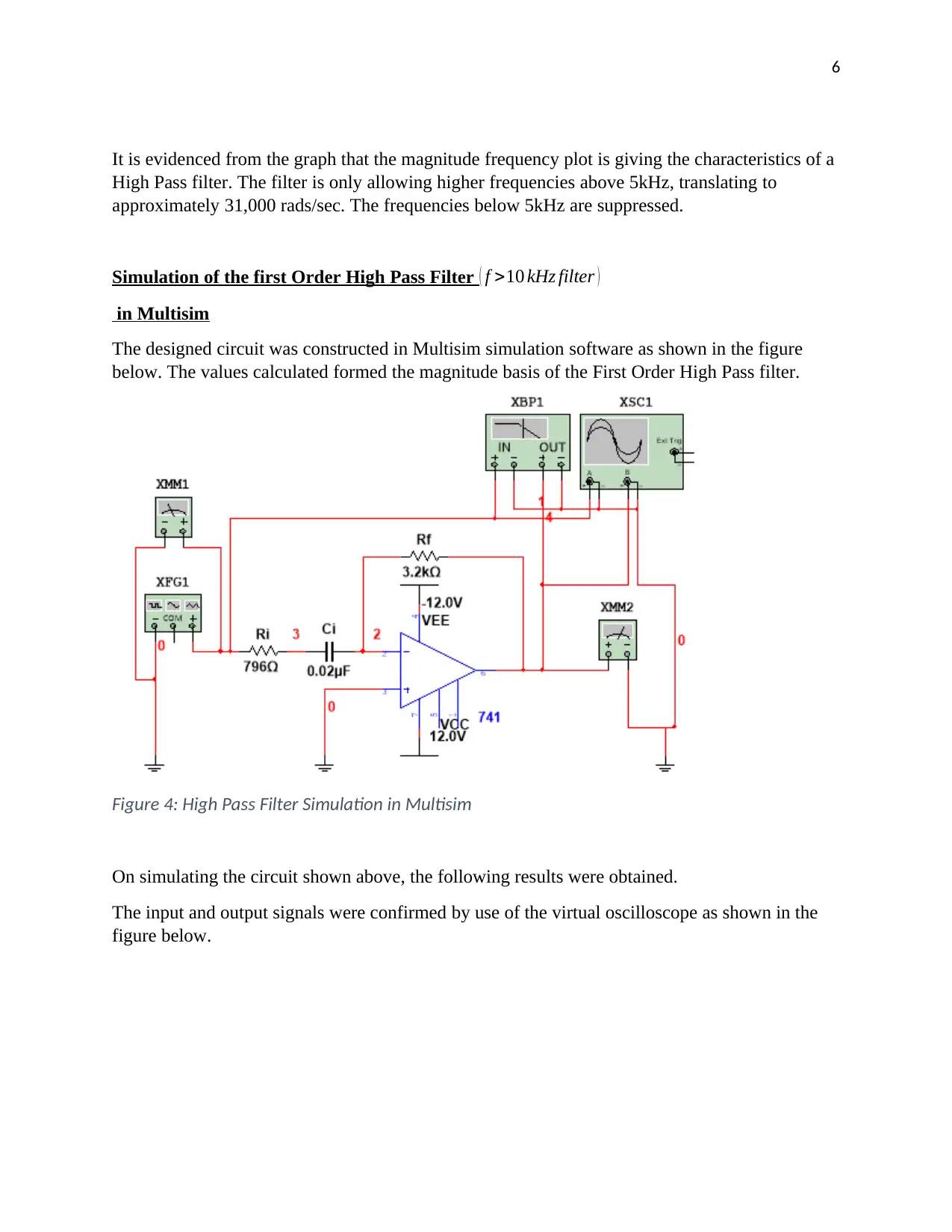
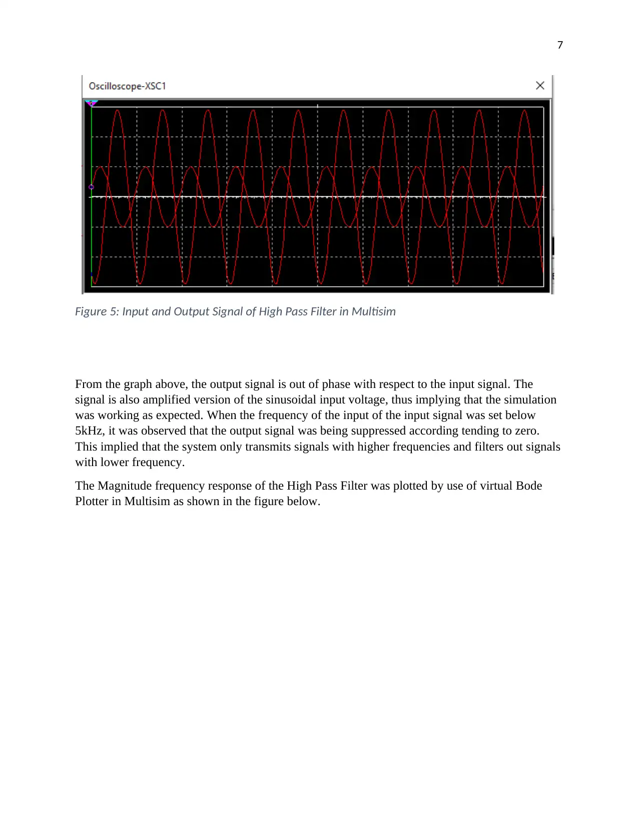
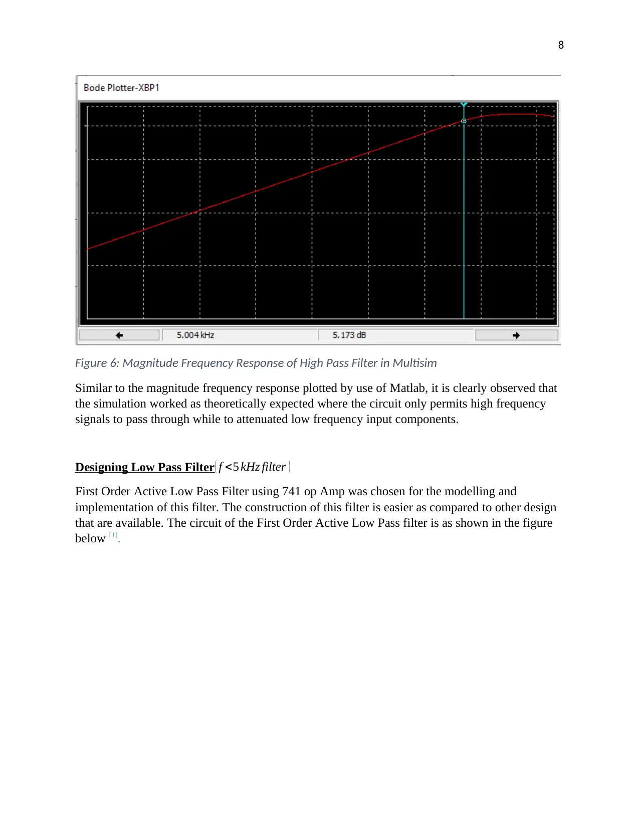
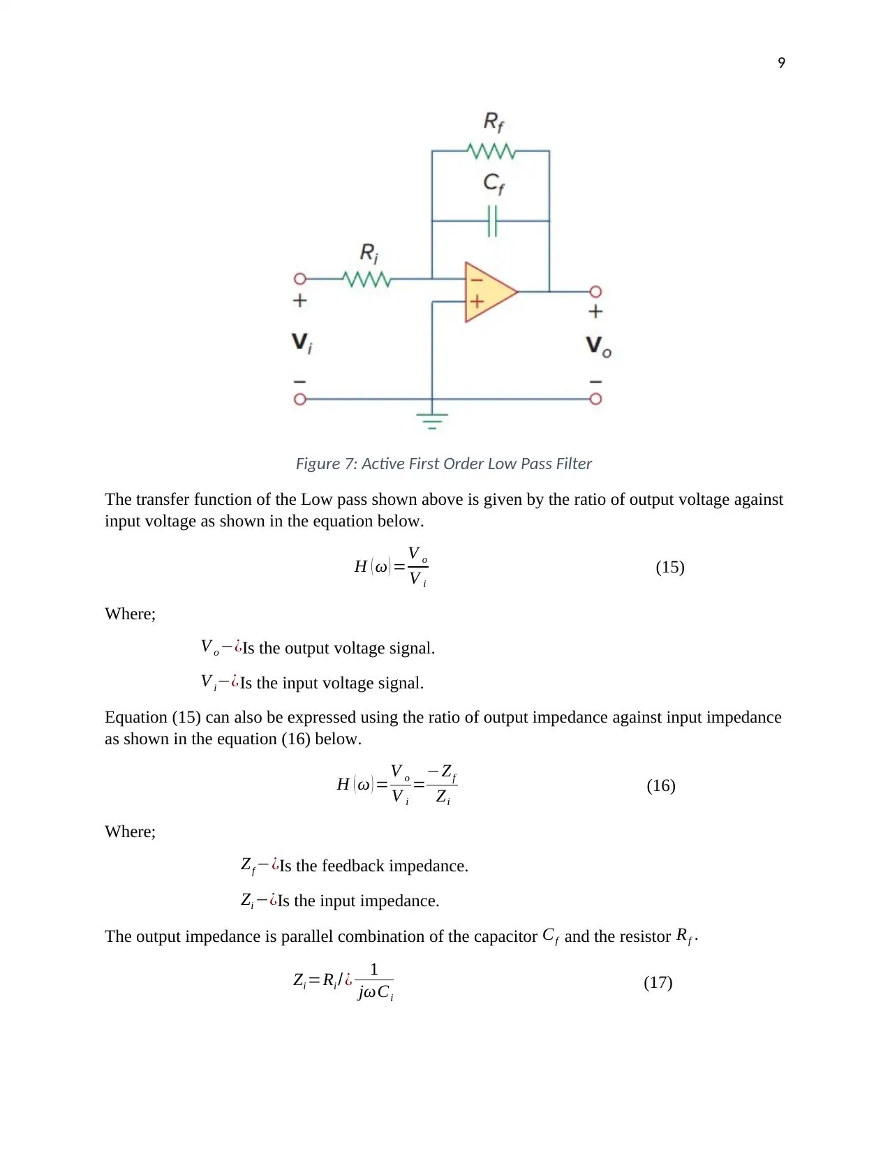
This report details the design and implementation of a 3-band audio amplifier, which functions as an audio equalizer. The design incorporates three filter types: a low-pass filter with a 5kHz cutoff, a band-pass filter with 5kHz and 10kHz corner frequencies, and a high-pass filter with a 5kHz corner frequency. The filters are cascaded with variable and summing amplifiers, with the variable gain amplifiers designed to operate between 0-40dB and the summing amplifier not exceeding 60dB. The design process involved stages of filter design, accompanied by Multisim simulations, and magnitude frequency plots of the filters' transfer functions were generated using MATLAB. The report includes detailed explanations of the design process for each filter, along with mathematical expressions, transfer functions, and simulation results. The report also presents the MATLAB code used for generating the magnitude frequency responses and provides graphical representations of the filters' performance characteristics.

1
3-BAND AUDIO AMPLIFIER
INTRODUCTION.
The objective of this report is to design a 3-band Audio Equalizer. The equalizer has three types
of filters combined. These filters include;
I. Low pass filter whose cut-off frequency is 5kHz.
II. Band pass filter whose corner frequencies are 5kHz and 10kHz.
III. High pass filter whose corner frequency is 5kHz.
The filters are cascaded together with the variable amplifier and summing amplifier as shown in
the schematic below.
Figure 1: Schematic diagram of 3-audio amplifier
The variable gain amplifiers are designed to operate between 0-40dB while the summing
amplifier ought to operate not more than 60dB. The audio speaker is represented by an 8Ω
resistor.
MODELLING OF THE 3-BAND AUDIO AMPLIFIER.
The design was done in stages as below. Implementation of the filter design stage is
accompanied by Multisim simulation. The magnitude frequency plot of the filters’ transfer
functions were done in Matlab software.
Designing of the High Pass Filter ( f >10 kHz filter )

2
First-order High Pass filter was designed using 741 op amp. This type of the filter was preferred
because it is simpler to construct with its underlying mathematical expressions. The filter is as
shown in the figure below [1].
Figure 2: First Order Active High Pass Filter
The transfer function of the First Order High pass filter is expressed as;
H ( ω ) =V o
V i
(1)
Where;
V o −¿Is the output voltage signal.
V i−¿Is the input voltage signal.
Equation (1) can also be expressed using the ratio of output impedance against input impedance
as shown in the equation (2) below.
H ( ω ) =V o
V i
=−Zf
Zi
(2)
Where;
Zf −¿Is the feedback impedance.
Zi −¿Is the input impedance.
The input impedance is series combination of the capacitor Ci and the resistor Ri .
Zi =Ri + 1
jωCi
(3)

3
The output impedance is basically the feedback resistor Rf
Substituting impedances in equation (2);
H ( ω ) = −Rf
Ri + 1
jω Ci
(4)
Rearranging equation (4) results to;
H ( ω ) = − jω Ci Rf
1+ jωCi Ri
(5)
As the frequency tend to infinity, the gain of the filter becomes;
H ( ω ) =lim ¿ ω → ∞ ( − jω Ci Rf
1+ jω Ci Ri ) =−Rf
Ri
(6)
The corner frequency of the First Order High Pass filter is given by;
ωc= 1
Ri Ci
(7)
Making Ri the subject of interest, then;
Ri= 1
ωc Ci
(8)
The cut-off frequency of the Low Pass filter at -3dB is specified as;
f c=10 kHz
Therefore,
ωc=2 π f c=2 π ( 10 , 00 0 Hz ) (9)
ωc=2 0,000 π Rads/sec
Selecting input capacitance as Ci=0. 02 μF , and substituting into equation (8);
Ri= 1
( 2 0,000 π ) ( 0. 02 ×10−6 F ) (10a)
Ri=795.77 Ω
The input resistance is therefore;
Ri=796 Ω (10b)
From equation (6), the D.C gain of the amplifier is given by;

4
H ( ω → ∞ )=−Rf
Ri
(11)
Setting the DC gain of the Low Pass Filter as;
|H ( ω → ∞ )|= Rf
Ri
=4 (12)
Then feedback resistance, Rf , is determined by;
Rf =4 Ri (13a)
Rf =5 ×796 Ω=3,183 Ω (13b)
The feedback resistance is therefore;
Rf =3.2 kΩ (14a)
Substituting the values in equation (5), the transfer function of the first Order High Pass Filter is
given by;
H ( ω ) = − jω ( 0.02 ×3.2 ×10−3 )
1+ jω ( 0.02×796 × 10−6 ) (14b)
Rewriting equation (14b) in complex s-domain;
jω=s
Then the transfer function is;
H ( s )= −s ( 0.02× 3.2×10−3 )
1+s ( 0.02× 796 ×10−6 ) (14c)
The magnitude frequency response of equation (14c) was drawn by help of MATLAB script as
shown below.
%------------------------------------------------------
%------START OF THE CODE-------------------------------
%The script calculates the transfer function of the
% First Order High Pass Filter and plots the
% Magnitude frequency response of the HPF
%-------------------------------------------------------
%------------------------------------------------------
clc;
clear all;
%-----------------------------------------------------
%-----Initializing Transfer Function------------------
s=tf('s');
%-----------------------------------------------------
%------------Transfer function of High Pass Filter----

5
H_hpf = s*(0.02*3.2*10^(-3))/(1+s*(0.02*796*10^(-6)))
%-----------------------------------------------------
%------Plotting Magnitude Frequency Response----------
%----------------------------------------------------
bode(H_hpf)
grid on
title('Magnitude Frequency Response')
xlabel('Frequency')
ylabel('Gain in dB')
%---------------------------------------------------
%---------END OF THE CODE---------------------------
Simplified transfer function of the first Order High Pass filter as computed in Matlab is;
H ( s )= ( 6.4 × 10−5 ) s
( 1.592× 10−5 ) s+1 (14d)
Or H ( jω ) = jω ( 6.4 × 10−5 )
jω ( 1.592 ×10−5 ) +1 (14e)
The magnitude frequency response of the first Order High Pass filter is as shown in the figure
below.
Figure 3: Magnitude Frequency Response of High Pass Filter

6
It is evidenced from the graph that the magnitude frequency plot is giving the characteristics of a
High Pass filter. The filter is only allowing higher frequencies above 5kHz, translating to
approximately 31,000 rads/sec. The frequencies below 5kHz are suppressed.
Simulation of the first Order High Pass Filter ( f >10 kHz filter )
in Multisim
The designed circuit was constructed in Multisim simulation software as shown in the figure
below. The values calculated formed the magnitude basis of the First Order High Pass filter.
Figure 4: High Pass Filter Simulation in Multisim
On simulating the circuit shown above, the following results were obtained.
The input and output signals were confirmed by use of the virtual oscilloscope as shown in the
figure below.

7
Figure 5: Input and Output Signal of High Pass Filter in Multisim
From the graph above, the output signal is out of phase with respect to the input signal. The
signal is also amplified version of the sinusoidal input voltage, thus implying that the simulation
was working as expected. When the frequency of the input of the input signal was set below
5kHz, it was observed that the output signal was being suppressed according tending to zero.
This implied that the system only transmits signals with higher frequencies and filters out signals
with lower frequency.
The Magnitude frequency response of the High Pass Filter was plotted by use of virtual Bode
Plotter in Multisim as shown in the figure below.

8
Figure 6: Magnitude Frequency Response of High Pass Filter in Multisim
Similar to the magnitude frequency response plotted by use of Matlab, it is clearly observed that
the simulation worked as theoretically expected where the circuit only permits high frequency
signals to pass through while to attenuated low frequency input components.
Designing Low Pass Filter ( f <5 kHz filter )
First Order Active Low Pass Filter using 741 op Amp was chosen for the modelling and
implementation of this filter. The construction of this filter is easier as compared to other design
that are available. The circuit of the First Order Active Low Pass filter is as shown in the figure
below [1].

9
Figure 7: Active First Order Low Pass Filter
The transfer function of the Low pass shown above is given by the ratio of output voltage against
input voltage as shown in the equation below.
H ( ω ) =V o
V i
(15)
Where;
V o −¿Is the output voltage signal.
V i−¿Is the input voltage signal.
Equation (15) can also be expressed using the ratio of output impedance against input impedance
as shown in the equation (16) below.
H ( ω ) =V o
V i
=−Zf
Zi
(16)
Where;
Zf −¿Is the feedback impedance.
Zi −¿Is the input impedance.
The output impedance is parallel combination of the capacitor Cf and the resistor Rf .
Zi =Ri /¿ 1
jωCi
(17)

10
Algebraically, the parallel combination of the impedance components in equation (17) is
expressed as;
Zi =
{ Ri /1
jωCi }
{ Ri + 1
jωCi } (18)
Simplifying equation (118);
Zi = Rf
1+ jωCf Rf
(19)
The input impedance is basically the feedback resistor Ri
Substituting impedances in equation (16), the transfer function of the First Order Low pass filter
is given as;
H ( ω ) =−Rf
Ri { 1
1+ jω Cf Rf } (20)
As the frequency tend to zero, the gain of the filter becomes;
H ( ω ) =lim ¿ ω → 0 ( −Rf
Ri { 1
1+ jωCf Rf })=−Rf
Ri
(21)
The corner frequency of the First Order Low Pass filter is given by;
ωc=ωc=2 π f c= 1
Rf Cf
(22)
But the corner frequency of the Low pass filter is specified as;
f c=5 kHz (23)
Selecting the value of the feedback capacitor as Cf =0.2 μF, then the feedback resistance as from
equation (22) is given by;
Rf = 1
2 π f c Cf
(24)
Substituting the values in equation (24);
Rf = 1
2 π ( 5000 Hz ) ( 0. 02 ×10−6 F ) (25a)
Rf =159 1.54 Ω (25b)
Therefore, the feedback resistance value is found to be;

11
Rf =1.6 kΩ (26)
From equation (21), the DC Low pass filter gain is given by;
H ( ω → 0 ) =−Rf
Ri
(27)
Assuming the DC gain of the Low pass filter is 4, i.e;
|H ( ω → 0 )|= Rf
Ri
=4 (28)
Then, the input resistance Ri is determined by;
Ri= Rf
4 (29a)
Ri= 1600 Ω
4 (29b)
Therefore, the input resistance of the Low Pass filter is;
Ri=400 Ω (30a)
Substituting the values in equation (20), the transfer function of the First Order Low pass filter is
as shown below.
H ( ω ) =−4 { 1
1+ jω ( 1.6 ×0.2 ×10−3 ) } (30b)
Rewriting equation (30b) in complex s-domain;
jω=s
Then the transfer function is;
H ( s )= { −4
1+ s ( 1.6 × 0.2× 10−3 ) } (30c)
The magnitude frequency response of equation (30c) was drawn by help of MATLAB script as
shown below.
%------------------------------------------------------
%------START OF THE CODE-------------------------------
%The script calculates the transfer function of the
% First Order Low Pass Filter and plots the
% Magnitude frequency response of the HPF
%-------------------------------------------------------
%------------------------------------------------------
clc;

12
clear all;
%-----------------------------------------------------
%-----Initializing Transfer Function------------------
s=tf('s');
%-----------------------------------------------------
%--------Transfer function of Low Pass Filter----
H_Lpf = -4/(1+s*(1.6*0.2*10^(-3)))
%-----------------------------------------------------
%------Plotting Magnitude Frequency Response----------
%----------------------------------------------------
bode(H_Lpf)
grid on
title('Magnitude Frequency Response of LPF')
xlabel('Frequency')
ylabel('Gain in dB')
%---------------------------------------------------
%---------END OF THE CODE---------------------------
Simplified transfer function of the first Order High Pass filter as computed in Matlab is;
H ( s )= −4
( 0.00032 ) s+ 1 (30d)
Or H ( jω ) = −4
Jω ( 0.00032 ) + 1 (30e)
The magnitude frequency response of the first Order High Pass filter is as shown in the figure
below.