ACC211 Report: ACC211 Project Evaluation for Auditizz Electronics

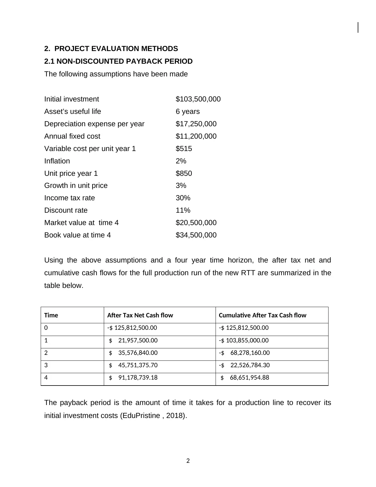
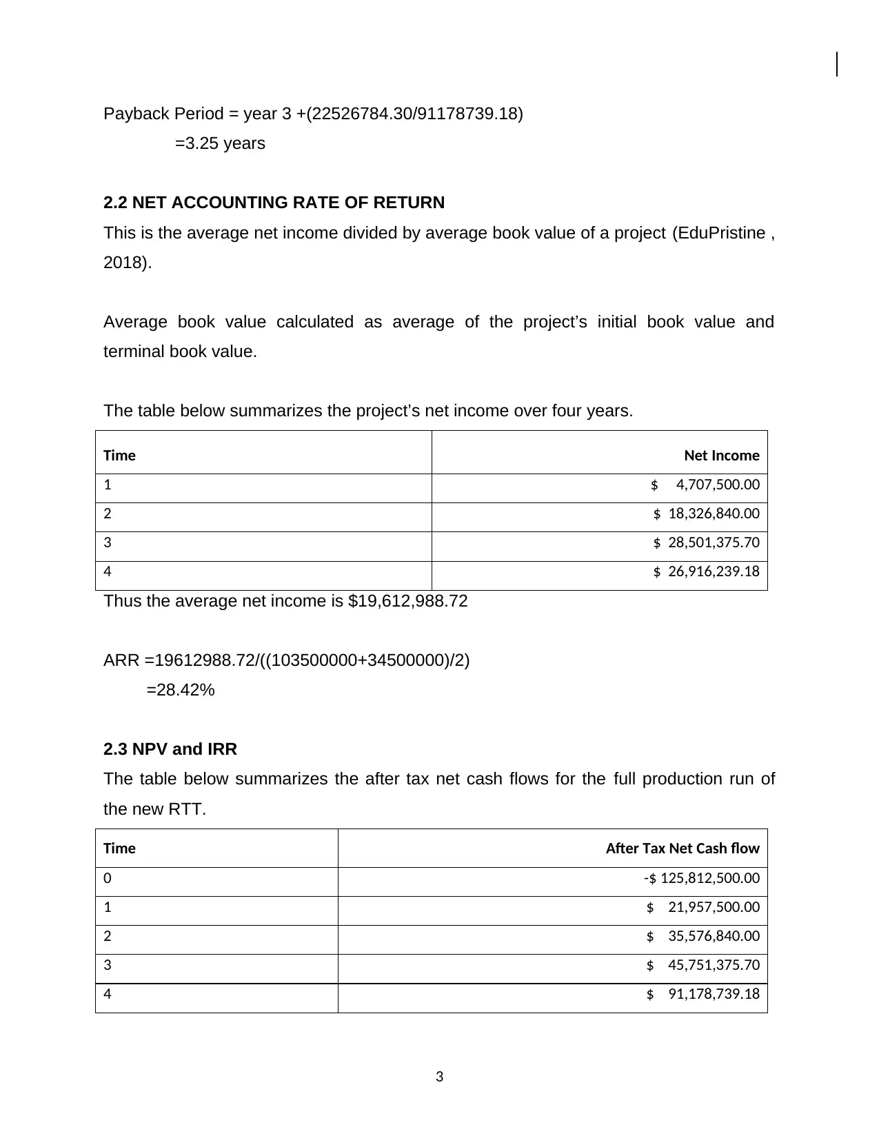
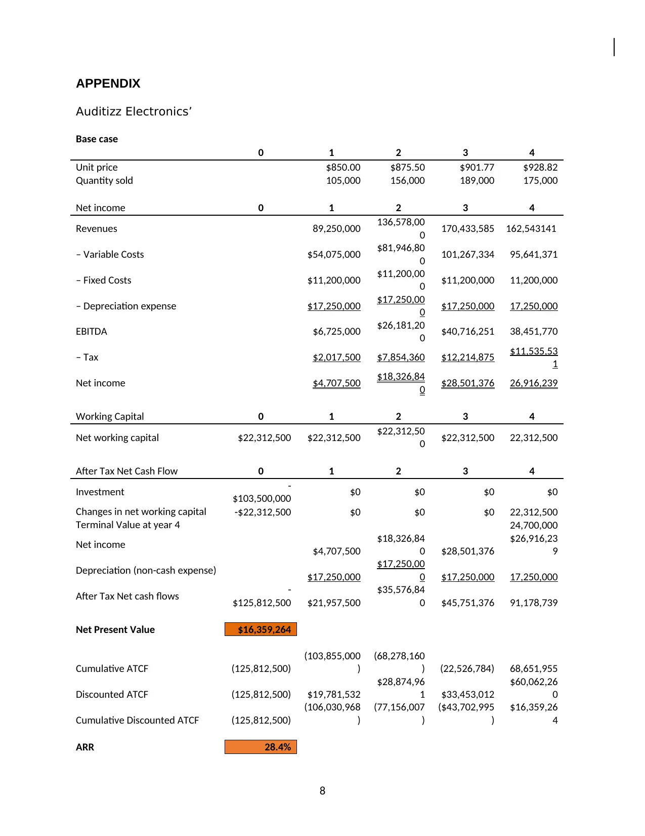
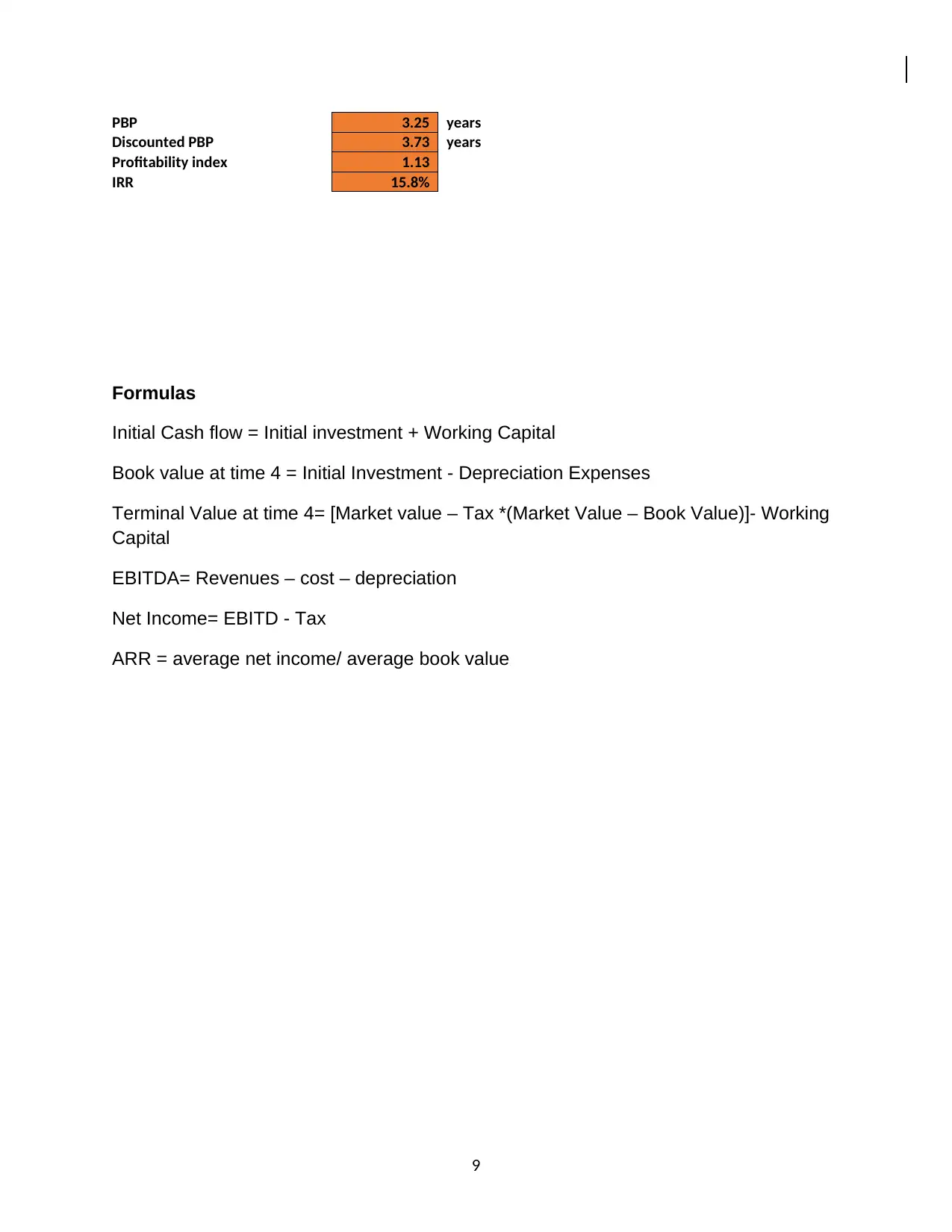
This report provides a comprehensive evaluation of Auditizz Electronics' potential investment in the production of real-time translators (RTT). The analysis employs both discounted and non-discounted cash flow methods to assess the project's viability. The report calculates the payback period, accounting rate of return (ARR), net present value (NPV), and internal rate of return (IRR). Sensitivity analyses are conducted to assess the impact of changes in unit price and sales quantity on the project's profitability. Forecasting risk and its implications are discussed. The report concludes with recommendations on whether Auditizz Electronics should proceed with the investment, considering the project's financial metrics, sensitivity to key assumptions, and overall forecasting risk. The efficient market hypothesis and the relationship between NPV and market value are also briefly addressed.

ACC211 REPORT PROJECT
Task 2

1. INTRODUCTION
In a bid to remain competitive, the CEO of Auditizz Electronics is considering an
investment into the production of ‘real-time translators’ (RTT) that will significantly
increase the company’s revenue.
The aim of the report is to give recommendations on whether Auditizz Electronics
should run a full production of the new RTT using both discounted and non-discounted
cash flow procedures.
Discounted and non-discounted cash flow methods may be used to evaluate the
viability of new projects such as a production line or investment in new equipment or
plant (Accounting Explained, 2019).
Discounted Cash flow methods calculate cash inflows and outflows during the assets
lifetime. These inflows and outflows are then discounted at the rate the company
expects to earn on their investment (Tucker, 2009).
There are several discounted cash flow methods. They are Internal Rate of Return (or
IRR), Discounted Payback Period (PBP) , Net Present Value (or NPV), and the
Profitability Index.
Non-discounted methods don’t consider the concept of the time value of money, hence
no discounting of cash flows. Examples of non-discounted valuation methods include
Payback Period and the Accounting Rate of Return (ARR).
1

2. PROJECT EVALUATION METHODS
2.1 NON-DISCOUNTED PAYBACK PERIOD
The following assumptions have been made
Initial investment $103,500,000
Asset’s useful life 6 years
Depreciation expense per year $17,250,000
Annual fixed cost $11,200,000
Variable cost per unit year 1 $515
Inflation 2%
Unit price year 1 $850
Growth in unit price 3%
Income tax rate 30%
Discount rate 11%
Market value at time 4 $20,500,000
Book value at time 4 $34,500,000
Using the above assumptions and a four year time horizon, the after tax net and
cumulative cash flows for the full production run of the new RTT are summarized in the
table below.
Time After Tax Net Cash flow Cumulative After Tax Cash flow
0 -$ 125,812,500.00 -$ 125,812,500.00
1 $ 21,957,500.00 -$ 103,855,000.00
2 $ 35,576,840.00 -$ 68,278,160.00
3 $ 45,751,375.70 -$ 22,526,784.30
4 $ 91,178,739.18 $ 68,651,954.88
The payback period is the amount of time it takes for a production line to recover its
initial investment costs (EduPristine , 2018).
2

Payback Period = year 3 +(22526784.30/91178739.18)
=3.25 years
2.2 NET ACCOUNTING RATE OF RETURN
This is the average net income divided by average book value of a project (EduPristine ,
2018).
Average book value calculated as average of the project’s initial book value and
terminal book value.
The table below summarizes the project’s net income over four years.
Time Net Income
1 $ 4,707,500.00
2 $ 18,326,840.00
3 $ 28,501,375.70
4 $ 26,916,239.18
Thus the average net income is $19,612,988.72
ARR =19612988.72/((103500000+34500000)/2)
=28.42%
2.3 NPV and IRR
The table below summarizes the after tax net cash flows for the full production run of
the new RTT.
Time After Tax Net Cash flow
0 -$ 125,812,500.00
1 $ 21,957,500.00
2 $ 35,576,840.00
3 $ 45,751,375.70
4 $ 91,178,739.18
3

The NPV is calculated using below formula where the discount rate is given as 11%.
NPV= -$ 125,812,500+ CF1*(1+r%)-1 + CF2*(1+r%)-2 + CF3*(1+r%)-3 + CF4*(1+r%)-4
=$16,359,264
The IRR is the rate at which the NPV equals zero .i.e.
0= -$ 125,812,500+ CF1*(1+i)-1 + CF2*(1+i)-2 + CF3*(1+i)-3 + CF4*(1+i)-4
Solving above equation, IRR is calculated as 15.8%.
2.4 SENSITIVITY ANALYSIS
Two sensitivity tests were investigated by varying the assumptions under the project’s
unit price and quantity sold.
Sensitivity One
In this case, it is assumed that the unit price of the new RTT drops from $850 to $800.
All other assumptions remain the same. Consequently, the calculated NPV drops to -
$608,283 following a small decrease in unit price.
Sensitivity Two
In this case, the quantity sold is assumed to be 15% less than expected. That is number
of units sold are 89,250 in Year 1; 132,600 units in Year 2; 160,650 units in Year 3; and
148,759 in Year 4. All other assumptions remain the same. Consequently, the
calculated NPV drops to -$419,230 when quantity sold are not met.
From the two sensitivity analyses, it is observed that the project’s success depends
largely on two assumptions- namely the assumption on quantities sold and unit prices.
This is because the project may be unprofitable if projected sold quantities are not
reached and/or the unit prices decerases slightly.
4

Forecasting Risk
This is the possibility that a company capital budgeting decision is not correct due to
errors in the projections. It is critical to understand the key inputs of any project that
could lead to a negative or positive NPV as this could affect whether a project will be
accepted or rejected (CourseBB, 2017).
A project can have a high forecasting risk following uncertainty of its key inputs.
Example of key inputs include volume of sales –a project may be accepted initially
however, if sales volumes are lower than expected the project may become
unacceptable. Other similarly key inputs include unit prices and/ or variable or fixed
costs.
2.5 RECOMMENDATIONS
The criteria as to whether a project should be accepted or rejected are as follows-
 If Payback period is smaller than the project’s useful life, accept it.
 If ARR is greater than company’s target rate, then accept project.
 If the NPV is positive, accept it since it is profitable.
 If the project’s IRR is bigger than the company’s cost of capital, accept the
project since it will be profitable.
Given that under the base scenario, the Payback is less than 4 years, the NPV is
positive, the ARR is large and the IRR is higher than 11%, then the project is feasible.
Therefore, it is recommended that Auditizz Electronics should invest into full production
of the ‘real-time translators’ (RTT).
However, managing forecasting risk is critical for Auditizz Electronics. From the
sensitivity analysis above, it was observed that the project has a high forecasting risk.
This is because if the quantities sold and/ or selling price reduces slightly, then the NPV
can drop to below zero thus making the project unprofitable. Hence these are key
assumptions that Auditizz Electronics should take into consideration when projecting its
future cash flows.
5

2.6 EFFICIENT MARKET HYPOTHESIS
The efficient market hypothesis (EMH) tells us that no investment strategy based on
either historical or current information produces extraordinary large returns. In other
words, a market is considered to be efficient is the current market value reflects all
public information. If a market is efficient with new information, then it cannot be used to
identify any positive NPV investment. However, if the market is not efficient then it is
possible to identify positive NPV investments (Windsor, 2019).
2.7 RELATIONSHIP BETWEEN NPV AND MARKET VALUE
A positive NPV suggests a project is profitable. Hence, it will increase the market value
to the company due to an increase revenue and shareholder value. On the other hand,
a negative NPV does not add value to a firm. In this case, a company should consider
other ways to invest the capital rather than investing in the project.
REFERENCES
Accounting Explained, 2019. Capital Budgeting. [Online]
Available at: http://accountingexplained.com/managerial/capital-budgeting/
6

CourseBB, 2017. How do you define Forecasting Risk?. [Online]
Available at: https://www.coursebb.com/2017/01/25/define-forecasting-risk/
EduPristine , 2018. Capital Budgeting: Techniques & Importance. [Online]
Available at: https://www.edupristine.com/blog/capital-budgeting-techniques
Tucker, J., 2009. How to set the hurdle rate for capital investments. [Online]
Available at: https://www.eprints.uwe.ac.uk/11334/1/Tucker_2009_QFinance_book_chapter.doc
Windsor, 2019. Efficient Market Hypothesis. [Online]
Available at: http://web2.uwindsor.ca/courses/business/assaf/Pmlect2a.pdf
7

APPENDIX
Auditizz Electronics’
Base case
0 1 2 3 4
Unit price $850.00 $875.50 $901.77 $928.82
Quantity sold 105,000 156,000 189,000 175,000
Net income 0 1 2 3 4
Revenues 89,250,000 136,578,00
0 170,433,585 162,543141
– Variable Costs $54,075,000 $81,946,80
0 101,267,334 95,641,371
– Fixed Costs $11,200,000 $11,200,00
0 $11,200,000 11,200,000
– Depreciation expense $17,250,000 $17,250,00
0 $17,250,000 17,250,000
EBITDA $6,725,000 $26,181,20
0 $40,716,251 38,451,770
– Tax $2,017,500 $7,854,360 $12,214,875 $11,535,53
1
Net income $4,707,500 $18,326,84
0 $28,501,376 26,916,239
Working Capital 0 1 2 3 4
Net working capital $22,312,500 $22,312,500 $22,312,50
0 $22,312,500 22,312,500
After Tax Net Cash Flow 0 1 2 3 4
Investment -
$103,500,000 $0 $0 $0 $0
Changes in net working capital -$22,312,500 $0 $0 $0 22,312,500
Terminal Value at year 4 24,700,000
Net income $4,707,500
$18,326,84
0 $28,501,376
$26,916,23
9
Depreciation (non-cash expense) $17,250,000
$17,250,00
0 $17,250,000 17,250,000
After Tax Net cash flows -
$125,812,500 $21,957,500
$35,576,84
0 $45,751,376 91,178,739
Net Present Value $16,359,264
Cumulative ATCF (125,812,500)
(103,855,000
)
(68,278,160
) (22,526,784) 68,651,955
Discounted ATCF (125,812,500) $19,781,532
$28,874,96
1 $33,453,012
$60,062,26
0
Cumulative Discounted ATCF (125,812,500)
(106,030,968
)
(77,156,007
)
($43,702,995
)
$16,359,26
4
ARR 28.4%
8

PBP 3.25 years
Discounted PBP 3.73 years
Profitability index 1.13
IRR 15.8%
Formulas
Initial Cash flow = Initial investment + Working Capital
Book value at time 4 = Initial Investment - Depreciation Expenses
Terminal Value at time 4= [Market value – Tax *(Market Value – Book Value)]- Working
Capital
EBITDA= Revenues – cost – depreciation
Net Income= EBITD - Tax
ARR = average net income/ average book value
9