Transport Economics: Regression Analysis of Air Passenger Travel
VerifiedAdded on 2023/06/15
|17
|2721
|299
Report
AI Summary
This report presents a comprehensive regression analysis of the factors influencing air passenger travel in Australia. The analysis uses data from 1970 to 2015 and examines the relationship between air passenger numbers (dependent variable Y) and independent variables such as GDP per capita (X1), international tourism departures (X2), international tourism arrivals (X3), and population (X4). The report includes scatter plots to visualize the association between variables, bivariate regression models to quantify the impact of each independent variable on air travel, and residual plots to test the linearity assumption of the regression models. Multiple regression models are also developed to assess the combined effect of different independent variables on air passenger travel. The findings highlight the statistical significance and explanatory power of GDP per capita, tourism numbers, and population in determining air travel demand in Australia.

Running Head: TRANSPORT ECONOMICS
Transport Economics
Name of the Student
Name of the University
Author note
Transport Economics
Name of the Student
Name of the University
Author note
Paraphrase This Document
Need a fresh take? Get an instant paraphrase of this document with our AI Paraphraser

1TRANSPORT ECONOMICS
Table of Contents
Task 1.........................................................................................................................................2
Task 2.........................................................................................................................................3
Bivariate regression................................................................................................................3
Residual plot...........................................................................................................................7
Task 3.........................................................................................................................................9
Model 1..................................................................................................................................9
Model 2................................................................................................................................11
Model 3....................................................................................................................................12
Task 4.......................................................................................................................................14
Forecast................................................................................................................................14
References................................................................................................................................16
2TRANSPORT ECONOMICS
Task 1
- 5,000,000 10,000,000 15,000,000 20,000,000 25,000,000
-
10,000,000
20,000,000
30,000,000
40,000,000
50,000,000
60,000,000
70,000,000
80,000,000
-
10,000,000
20,000,000
30,000,000
40,000,000
50,000,000
60,000,000
70,000,000
80,000,000
f(x) = 922.330951872083 x + 2851837.16103047
R² = 0.977320752162377 f(x) = 5.87873434629525 x − 74877468.3237875
R² = 0.945320839513967
R² = 0R² = 0
Scatter Plot
International tourism, number of departures (X2)
Linear (International tourism, number of departures (X2))
International tourism, number of arrivals (X3)
Linear (International tourism, number of arrivals (X3))
Population (X4)
Linear (Population (X4))
GDP per capita (X1)
Linear (GDP per capita (X1))
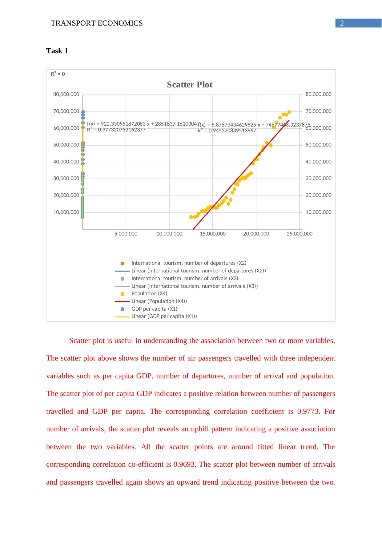
Scatter plot is useful in understanding the association between two or more variables.
The scatter plot above shows the number of air passengers travelled with three independent
variables such as per capita GDP, number of departures, number of arrival and population.
The scatter plot of per capita GDP indicates a positive relation between number of passengers
travelled and GDP per capita. The corresponding correlation coefficient is 0.9773. For
number of arrivals, the scatter plot reveals an uphill pattern indicating a positive association
between the two variables. All the scatter points are around fitted linear trend. The
corresponding correlation co-efficient is 0.9693. The scatter plot between number of arrivals
and passengers travelled again shows an upward trend indicating positive between the two.
Task 1
- 5,000,000 10,000,000 15,000,000 20,000,000 25,000,000
-
10,000,000
20,000,000
30,000,000
40,000,000
50,000,000
60,000,000
70,000,000
80,000,000
-
10,000,000
20,000,000
30,000,000
40,000,000
50,000,000
60,000,000
70,000,000
80,000,000
f(x) = 922.330951872083 x + 2851837.16103047
R² = 0.977320752162377 f(x) = 5.87873434629525 x − 74877468.3237875
R² = 0.945320839513967
R² = 0R² = 0
Scatter Plot
International tourism, number of departures (X2)
Linear (International tourism, number of departures (X2))
International tourism, number of arrivals (X3)
Linear (International tourism, number of arrivals (X3))
Population (X4)
Linear (Population (X4))
GDP per capita (X1)
Linear (GDP per capita (X1))
Scatter plot is useful in understanding the association between two or more variables.
The scatter plot above shows the number of air passengers travelled with three independent
variables such as per capita GDP, number of departures, number of arrival and population.
The scatter plot of per capita GDP indicates a positive relation between number of passengers
travelled and GDP per capita. The corresponding correlation coefficient is 0.9773. For
number of arrivals, the scatter plot reveals an uphill pattern indicating a positive association
between the two variables. All the scatter points are around fitted linear trend. The
corresponding correlation co-efficient is 0.9693. The scatter plot between number of arrivals
and passengers travelled again shows an upward trend indicating positive between the two.
⊘ This is a preview!⊘
Do you want full access?
Subscribe today to unlock all pages.
Trusted by 1+ million students worldwide
3TRANSPORT ECONOMICS
Population also has a positive relation with passengers travelled. Therefore, all the variables
have a linear relationship with the dependent variables. Scatter plot however shows only
degree of association (Fox, 2015). It does not indicate any cause and effect relation. For the
later, a regression needs to be done.
Task 2
Bivariate regression
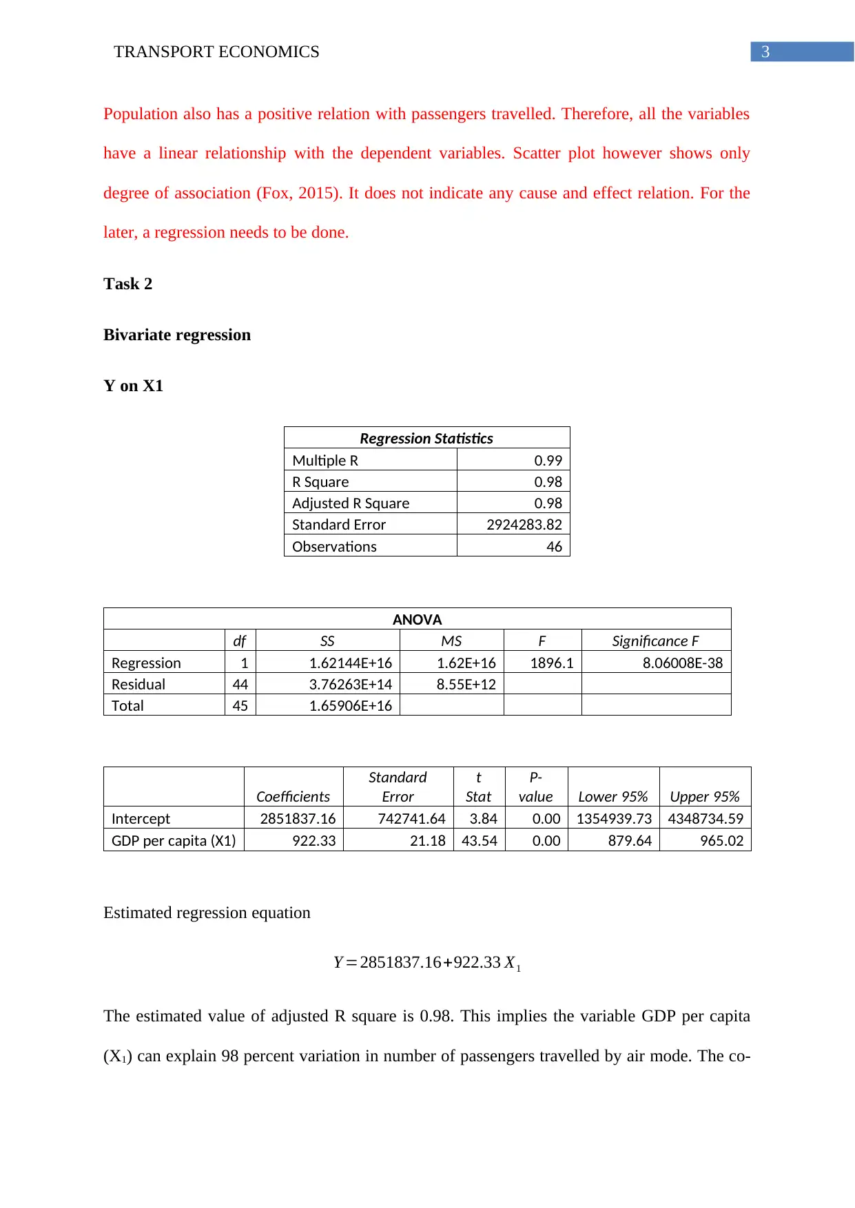
Y on X1
Regression Statistics
Multiple R 0.99
R Square 0.98
Adjusted R Square 0.98
Standard Error 2924283.82
Observations 46
ANOVA
df SS MS F Significance F
Regression 1 1.62144E+16 1.62E+16 1896.1 8.06008E-38
Residual 44 3.76263E+14 8.55E+12
Total 45 1.65906E+16
Coefficients
Standard
Error
t
Stat
P-
value Lower 95% Upper 95%
Intercept 2851837.16 742741.64 3.84 0.00 1354939.73 4348734.59
GDP per capita (X1) 922.33 21.18 43.54 0.00 879.64 965.02
Estimated regression equation
Y =2851837.16+922.33 X1
The estimated value of adjusted R square is 0.98. This implies the variable GDP per capita
(X1) can explain 98 percent variation in number of passengers travelled by air mode. The co-
Population also has a positive relation with passengers travelled. Therefore, all the variables
have a linear relationship with the dependent variables. Scatter plot however shows only
degree of association (Fox, 2015). It does not indicate any cause and effect relation. For the
later, a regression needs to be done.
Task 2
Bivariate regression
Y on X1
Regression Statistics
Multiple R 0.99
R Square 0.98
Adjusted R Square 0.98
Standard Error 2924283.82
Observations 46
ANOVA
df SS MS F Significance F
Regression 1 1.62144E+16 1.62E+16 1896.1 8.06008E-38
Residual 44 3.76263E+14 8.55E+12
Total 45 1.65906E+16
Coefficients
Standard
Error
t
Stat
P-
value Lower 95% Upper 95%
Intercept 2851837.16 742741.64 3.84 0.00 1354939.73 4348734.59
GDP per capita (X1) 922.33 21.18 43.54 0.00 879.64 965.02
Estimated regression equation
Y =2851837.16+922.33 X1
The estimated value of adjusted R square is 0.98. This implies the variable GDP per capita
(X1) can explain 98 percent variation in number of passengers travelled by air mode. The co-
Paraphrase This Document
Need a fresh take? Get an instant paraphrase of this document with our AI Paraphraser
4TRANSPORT ECONOMICS
efficient of X1 is 934.64. The positive value of the coefficient implies that GDP per capita has
a positive impact on passengers travelled. The corresponding p value for the co-efficient is
0.00. The p value less than significance level (0.05) means the variable is statistically
significant at the corresponding level of significance. The high value of R square along with a
significant p value implies the model is best fitted for the given variables.
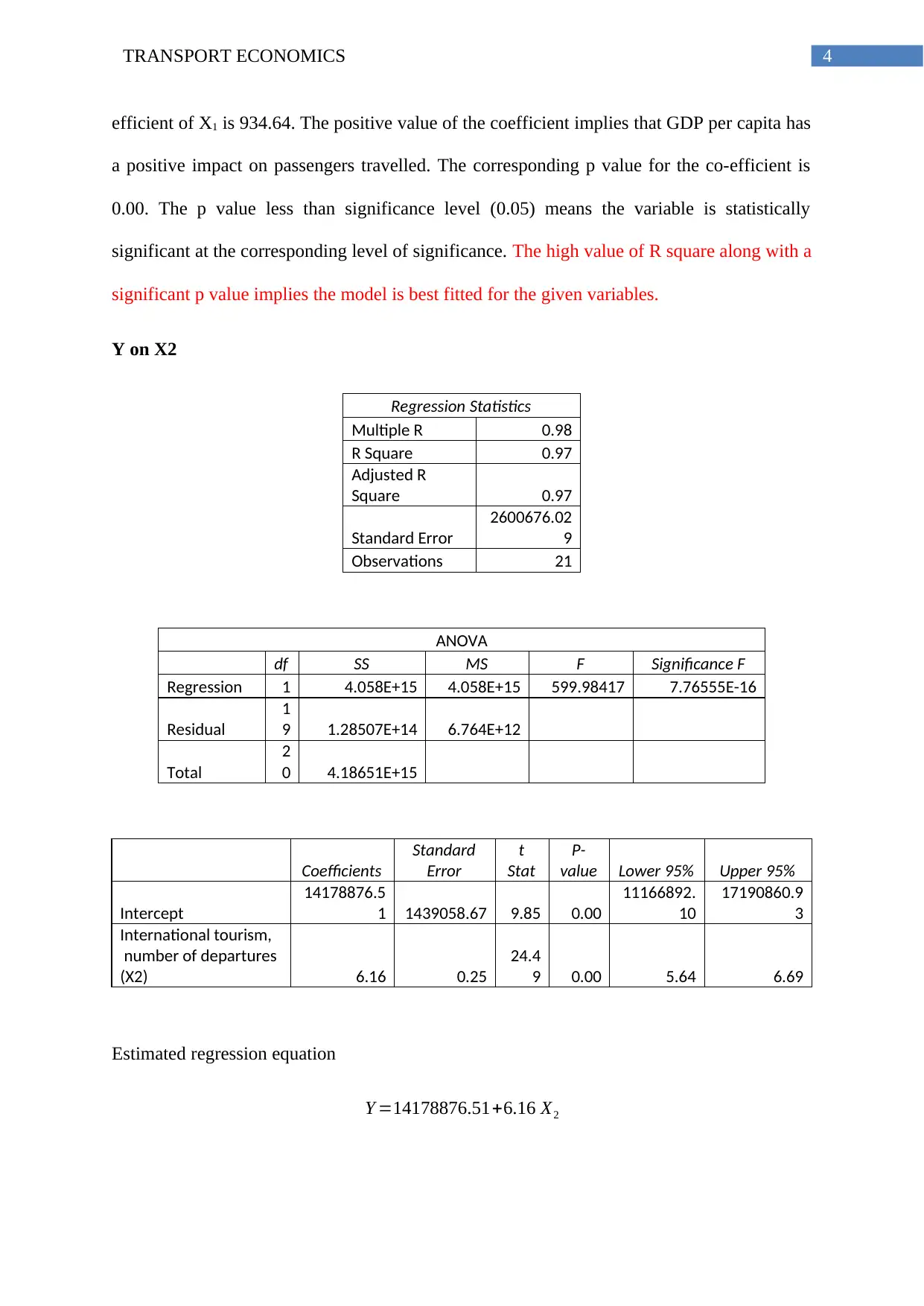
Y on X2
Regression Statistics
Multiple R 0.98
R Square 0.97
Adjusted R
Square 0.97
Standard Error
2600676.02
9
Observations 21
ANOVA
df SS MS F Significance F
Regression 1 4.058E+15 4.058E+15 599.98417 7.76555E-16
Residual
1
9 1.28507E+14 6.764E+12
Total
2
0 4.18651E+15
Coefficients
Standard
Error
t
Stat
P-
value Lower 95% Upper 95%
Intercept
14178876.5
1 1439058.67 9.85 0.00
11166892.
10
17190860.9
3
International tourism,
number of departures
(X2) 6.16 0.25
24.4
9 0.00 5.64 6.69
Estimated regression equation
Y =14178876.51+6.16 X2
efficient of X1 is 934.64. The positive value of the coefficient implies that GDP per capita has
a positive impact on passengers travelled. The corresponding p value for the co-efficient is
0.00. The p value less than significance level (0.05) means the variable is statistically
significant at the corresponding level of significance. The high value of R square along with a
significant p value implies the model is best fitted for the given variables.
Y on X2
Regression Statistics
Multiple R 0.98
R Square 0.97
Adjusted R
Square 0.97
Standard Error
2600676.02
9
Observations 21
ANOVA
df SS MS F Significance F
Regression 1 4.058E+15 4.058E+15 599.98417 7.76555E-16
Residual
1
9 1.28507E+14 6.764E+12
Total
2
0 4.18651E+15
Coefficients
Standard
Error
t
Stat
P-
value Lower 95% Upper 95%
Intercept
14178876.5
1 1439058.67 9.85 0.00
11166892.
10
17190860.9
3
International tourism,
number of departures
(X2) 6.16 0.25
24.4
9 0.00 5.64 6.69
Estimated regression equation
Y =14178876.51+6.16 X2
5TRANSPORT ECONOMICS
The estimated value of adjusted R square is 0.97. This implies the variable; number of
departure (X2) can explain 97 percent variation in number of passengers travelled by air
mode. The co-efficient of X1 is 6.16. As most of the variation in the dependent variable is
explained by the independent variable, the model is good fit model. The positive value of the
coefficient implies that number of departure has a positive impact on passengers travelled.
The corresponding p value for the co-efficient is 0.00. The p value less than significance level
(0.05) means the variable is statistically significant at the corresponding level of significance.
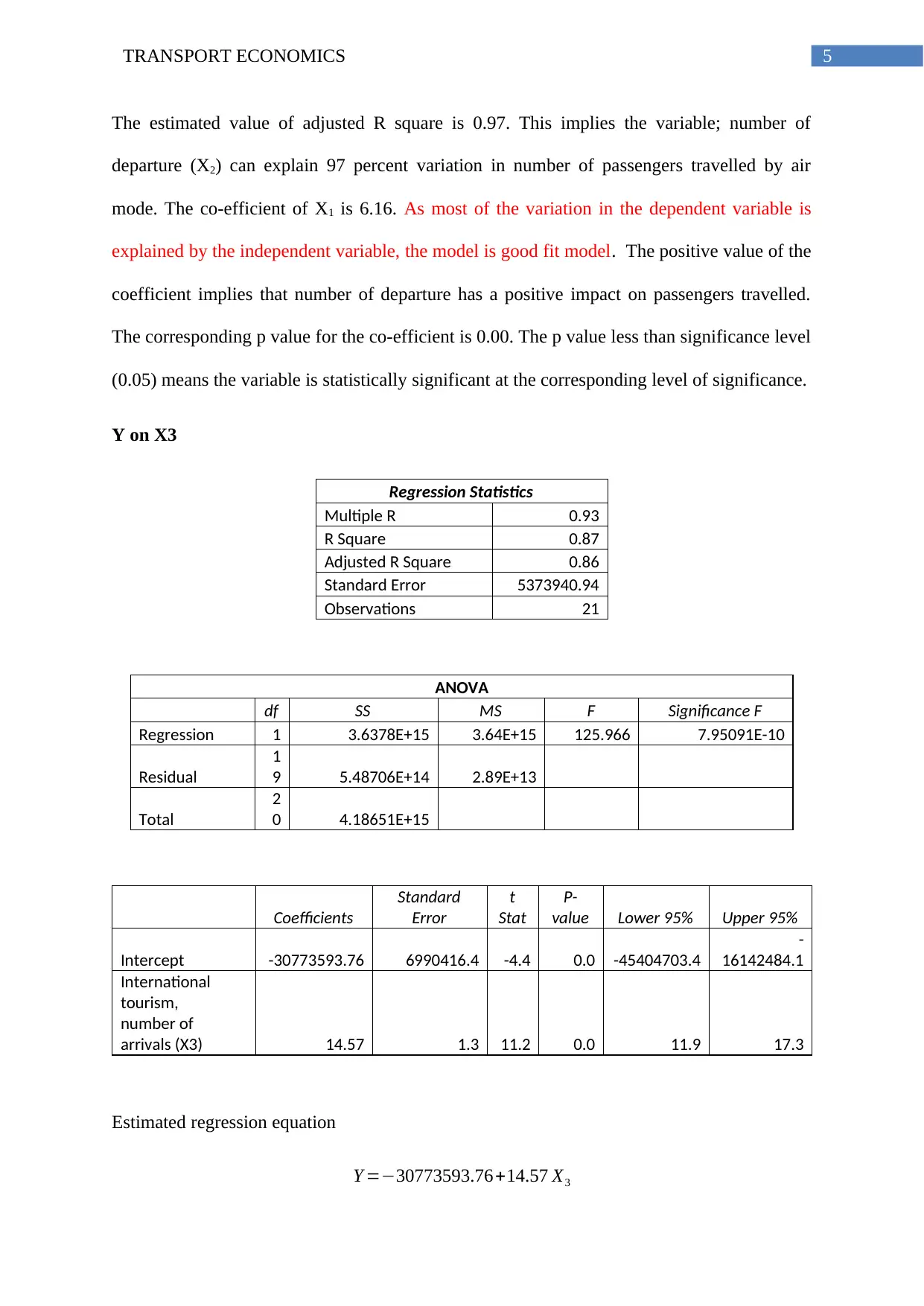
Y on X3
Regression Statistics
Multiple R 0.93
R Square 0.87
Adjusted R Square 0.86
Standard Error 5373940.94
Observations 21
ANOVA
df SS MS F Significance F
Regression 1 3.6378E+15 3.64E+15 125.966 7.95091E-10
Residual
1
9 5.48706E+14 2.89E+13
Total
2
0 4.18651E+15
Coefficients
Standard
Error
t
Stat
P-
value Lower 95% Upper 95%
Intercept -30773593.76 6990416.4 -4.4 0.0 -45404703.4
-
16142484.1
International
tourism,
number of
arrivals (X3) 14.57 1.3 11.2 0.0 11.9 17.3
Estimated regression equation
Y =−30773593.76+14.57 X3
The estimated value of adjusted R square is 0.97. This implies the variable; number of
departure (X2) can explain 97 percent variation in number of passengers travelled by air
mode. The co-efficient of X1 is 6.16. As most of the variation in the dependent variable is
explained by the independent variable, the model is good fit model. The positive value of the
coefficient implies that number of departure has a positive impact on passengers travelled.
The corresponding p value for the co-efficient is 0.00. The p value less than significance level
(0.05) means the variable is statistically significant at the corresponding level of significance.
Y on X3
Regression Statistics
Multiple R 0.93
R Square 0.87
Adjusted R Square 0.86
Standard Error 5373940.94
Observations 21
ANOVA
df SS MS F Significance F
Regression 1 3.6378E+15 3.64E+15 125.966 7.95091E-10
Residual
1
9 5.48706E+14 2.89E+13
Total
2
0 4.18651E+15
Coefficients
Standard
Error
t
Stat
P-
value Lower 95% Upper 95%
Intercept -30773593.76 6990416.4 -4.4 0.0 -45404703.4
-
16142484.1
International
tourism,
number of
arrivals (X3) 14.57 1.3 11.2 0.0 11.9 17.3
Estimated regression equation
Y =−30773593.76+14.57 X3
⊘ This is a preview!⊘
Do you want full access?
Subscribe today to unlock all pages.
Trusted by 1+ million students worldwide
6TRANSPORT ECONOMICS
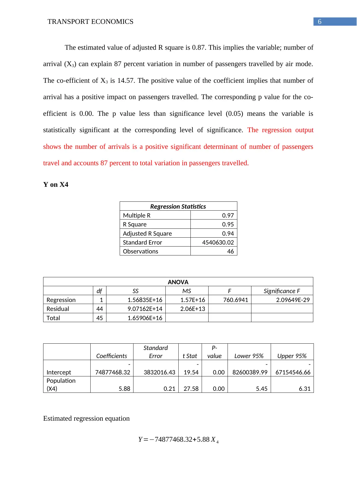
The estimated value of adjusted R square is 0.87. This implies the variable; number of
arrival (X3) can explain 87 percent variation in number of passengers travelled by air mode.
The co-efficient of X3 is 14.57. The positive value of the coefficient implies that number of
arrival has a positive impact on passengers travelled. The corresponding p value for the co-
efficient is 0.00. The p value less than significance level (0.05) means the variable is
statistically significant at the corresponding level of significance. The regression output
shows the number of arrivals is a positive significant determinant of number of passengers
travel and accounts 87 percent to total variation in passengers travelled.
Y on X4
Regression Statistics
Multiple R 0.97
R Square 0.95
Adjusted R Square 0.94
Standard Error 4540630.02
Observations 46
ANOVA
df SS MS F Significance F
Regression 1 1.56835E+16 1.57E+16 760.6941 2.09649E-29
Residual 44 9.07162E+14 2.06E+13
Total 45 1.65906E+16
Coefficients
Standard
Error t Stat
P-
value Lower 95% Upper 95%
Intercept
-
74877468.32 3832016.43
-
19.54 0.00
-
82600389.99
-
67154546.66
Population
(X4) 5.88 0.21 27.58 0.00 5.45 6.31
Estimated regression equation
Y =−74877468.32+5.88 X 4
Paraphrase This Document
Need a fresh take? Get an instant paraphrase of this document with our AI Paraphraser
7TRANSPORT ECONOMICS
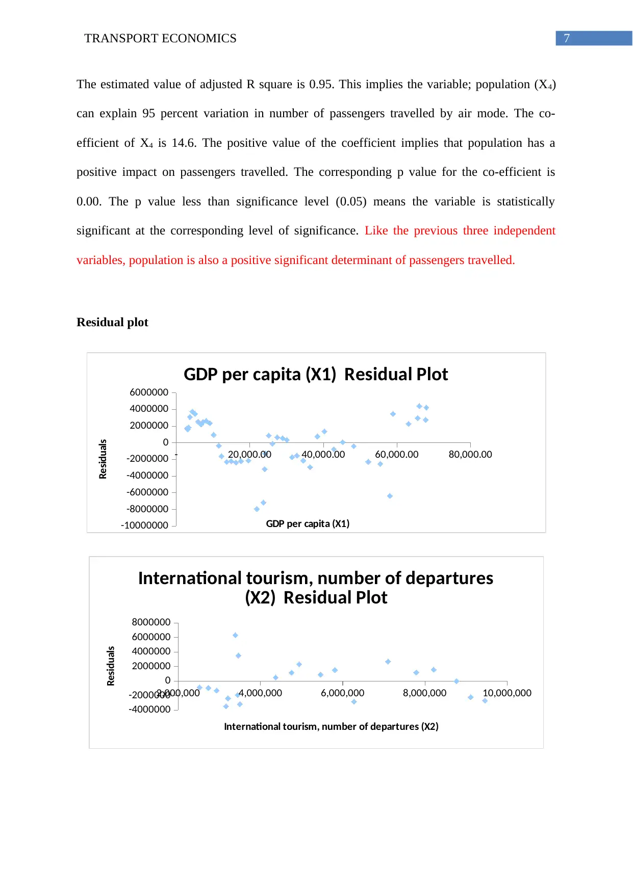
The estimated value of adjusted R square is 0.95. This implies the variable; population (X4)
can explain 95 percent variation in number of passengers travelled by air mode. The co-
efficient of X4 is 14.6. The positive value of the coefficient implies that population has a
positive impact on passengers travelled. The corresponding p value for the co-efficient is
0.00. The p value less than significance level (0.05) means the variable is statistically
significant at the corresponding level of significance. Like the previous three independent
variables, population is also a positive significant determinant of passengers travelled.
Residual plot
- 20,000.00 40,000.00 60,000.00 80,000.00
-10000000
-8000000
-6000000
-4000000
-2000000
0
2000000
4000000
6000000
GDP per capita (X1) Residual Plot
GDP per capita (X1)
Residuals
2,000,000 4,000,000 6,000,000 8,000,000 10,000,000
-4000000
-2000000
0
2000000
4000000
6000000
8000000
International tourism, number of departures
(X2) Residual Plot
International tourism, number of departures (X2)
Residuals
8TRANSPORT ECONOMICS
3,000,000 4,000,000 5,000,000 6,000,000 7,000,000 8,000,000
-10000000
-5000000
0
5000000
10000000
15000000
International tourism, number of
arrivals (X3) Residual Plot
International tourism, number of arrivals (X3)
Residuals
10,000,000 15,000,000 20,000,000 25,000,000
-10000000
-5000000
0
5000000
10000000
Population (X4) Residual Plot
Population (X4)
Residuals
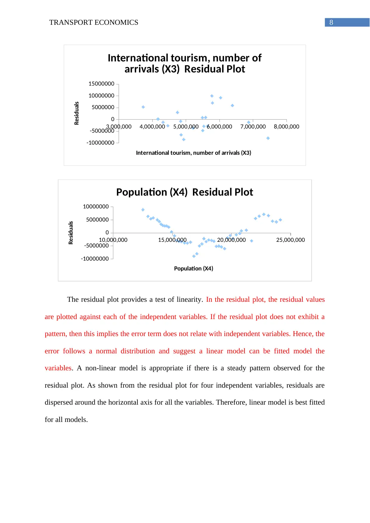
The residual plot provides a test of linearity. In the residual plot, the residual values
are plotted against each of the independent variables. If the residual plot does not exhibit a
pattern, then this implies the error term does not relate with independent variables. Hence, the
error follows a normal distribution and suggest a linear model can be fitted model the
variables. A non-linear model is appropriate if there is a steady pattern observed for the
residual plot. As shown from the residual plot for four independent variables, residuals are
dispersed around the horizontal axis for all the variables. Therefore, linear model is best fitted
for all models.
3,000,000 4,000,000 5,000,000 6,000,000 7,000,000 8,000,000
-10000000
-5000000
0
5000000
10000000
15000000
International tourism, number of
arrivals (X3) Residual Plot
International tourism, number of arrivals (X3)
Residuals
10,000,000 15,000,000 20,000,000 25,000,000
-10000000
-5000000
0
5000000
10000000
Population (X4) Residual Plot
Population (X4)
Residuals
The residual plot provides a test of linearity. In the residual plot, the residual values
are plotted against each of the independent variables. If the residual plot does not exhibit a
pattern, then this implies the error term does not relate with independent variables. Hence, the
error follows a normal distribution and suggest a linear model can be fitted model the
variables. A non-linear model is appropriate if there is a steady pattern observed for the
residual plot. As shown from the residual plot for four independent variables, residuals are
dispersed around the horizontal axis for all the variables. Therefore, linear model is best fitted
for all models.
⊘ This is a preview!⊘
Do you want full access?
Subscribe today to unlock all pages.
Trusted by 1+ million students worldwide
9TRANSPORT ECONOMICS
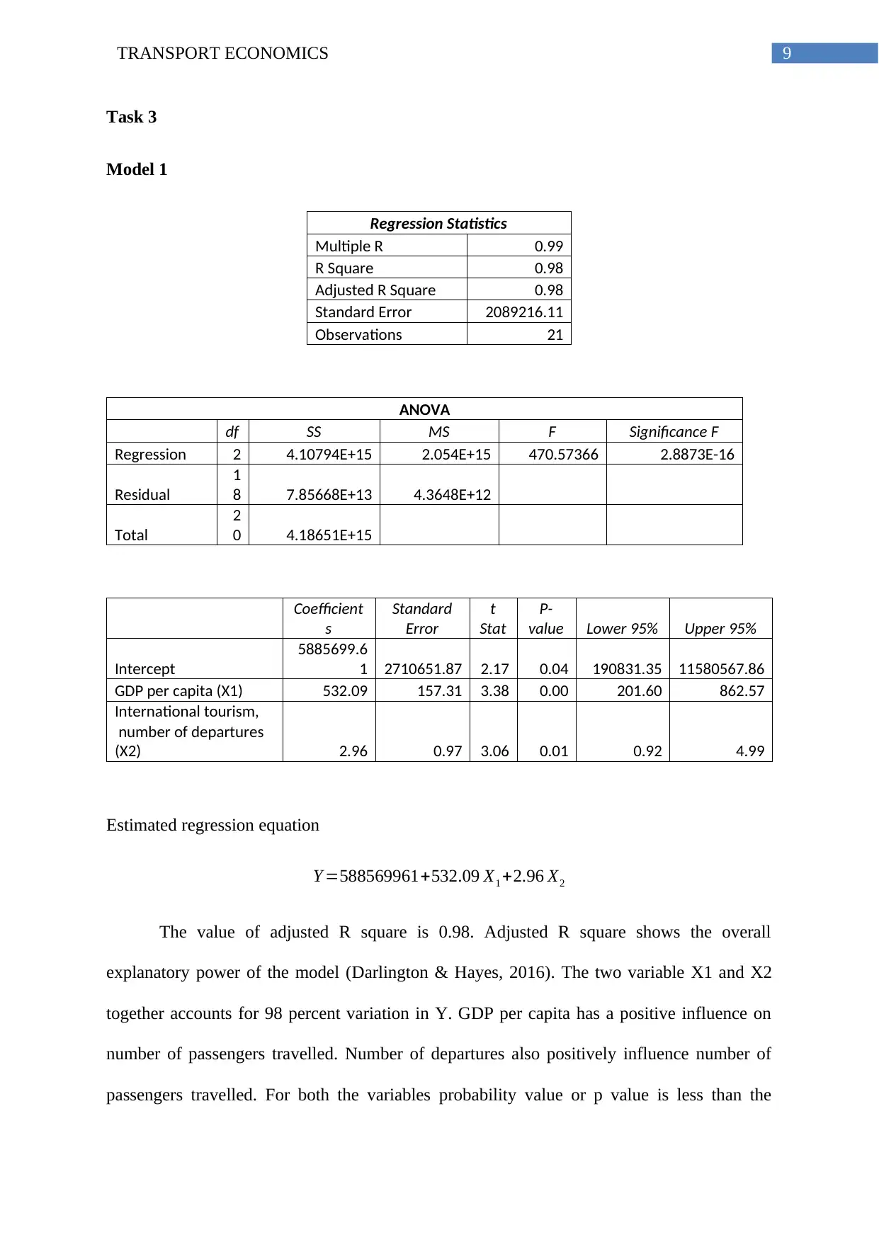
Task 3
Model 1
Regression Statistics
Multiple R 0.99
R Square 0.98
Adjusted R Square 0.98
Standard Error 2089216.11
Observations 21
ANOVA
df SS MS F Significance F
Regression 2 4.10794E+15 2.054E+15 470.57366 2.8873E-16
Residual
1
8 7.85668E+13 4.3648E+12
Total
2
0 4.18651E+15
Coefficient
s
Standard
Error
t
Stat
P-
value Lower 95% Upper 95%
Intercept
5885699.6
1 2710651.87 2.17 0.04 190831.35 11580567.86
GDP per capita (X1) 532.09 157.31 3.38 0.00 201.60 862.57
International tourism,
number of departures
(X2) 2.96 0.97 3.06 0.01 0.92 4.99
Estimated regression equation
Y =588569961+532.09 X1 +2.96 X2
The value of adjusted R square is 0.98. Adjusted R square shows the overall
explanatory power of the model (Darlington & Hayes, 2016). The two variable X1 and X2
together accounts for 98 percent variation in Y. GDP per capita has a positive influence on
number of passengers travelled. Number of departures also positively influence number of
passengers travelled. For both the variables probability value or p value is less than the
Paraphrase This Document
Need a fresh take? Get an instant paraphrase of this document with our AI Paraphraser
10TRANSPORT ECONOMICS
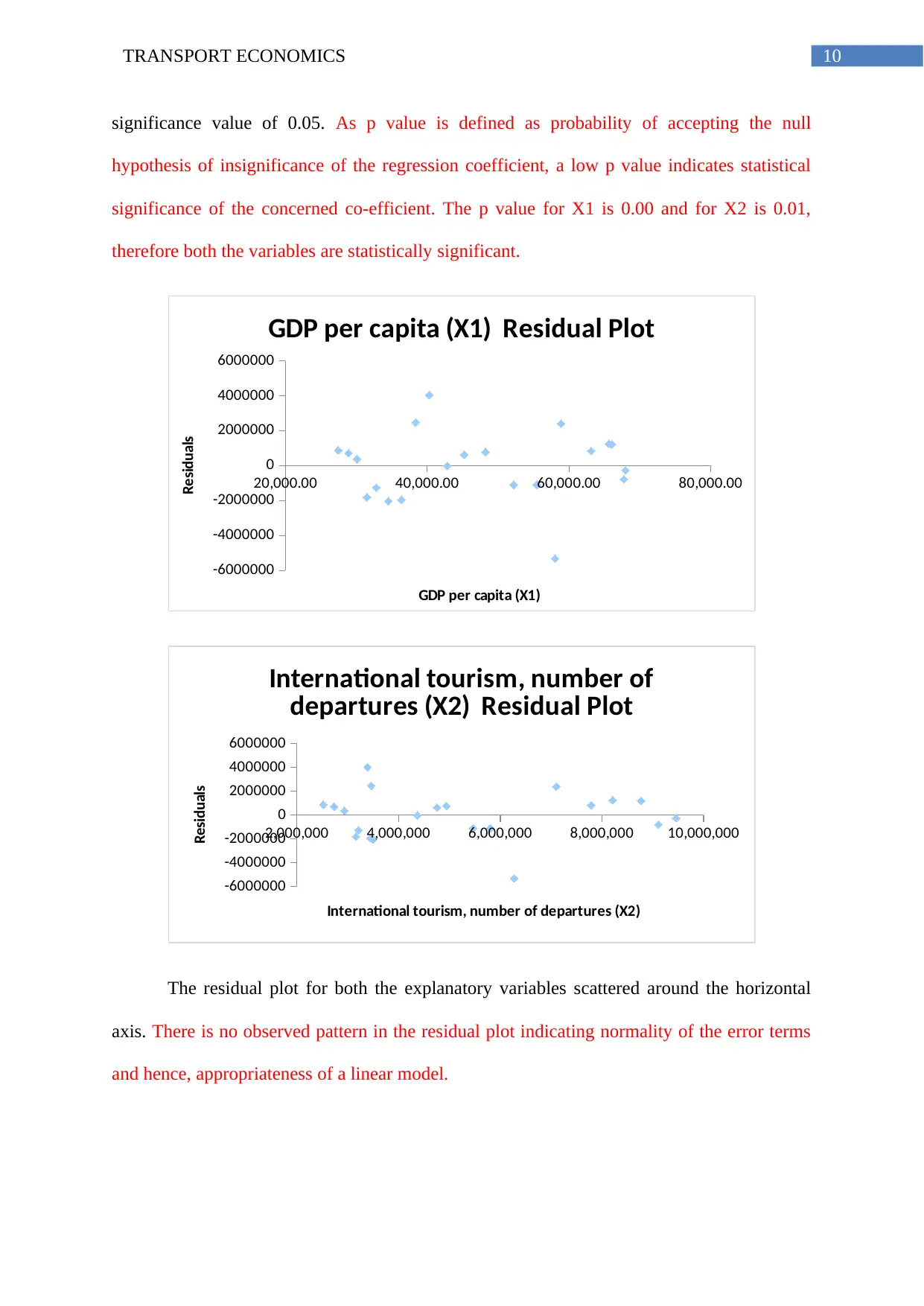
significance value of 0.05. As p value is defined as probability of accepting the null
hypothesis of insignificance of the regression coefficient, a low p value indicates statistical
significance of the concerned co-efficient. The p value for X1 is 0.00 and for X2 is 0.01,
therefore both the variables are statistically significant.
20,000.00 40,000.00 60,000.00 80,000.00
-6000000
-4000000
-2000000
0
2000000
4000000
6000000
GDP per capita (X1) Residual Plot
GDP per capita (X1)
Residuals
2,000,000 4,000,000 6,000,000 8,000,000 10,000,000
-6000000
-4000000
-2000000
0
2000000
4000000
6000000
International tourism, number of
departures (X2) Residual Plot
International tourism, number of departures (X2)
Residuals
The residual plot for both the explanatory variables scattered around the horizontal
axis. There is no observed pattern in the residual plot indicating normality of the error terms
and hence, appropriateness of a linear model.
11TRANSPORT ECONOMICS
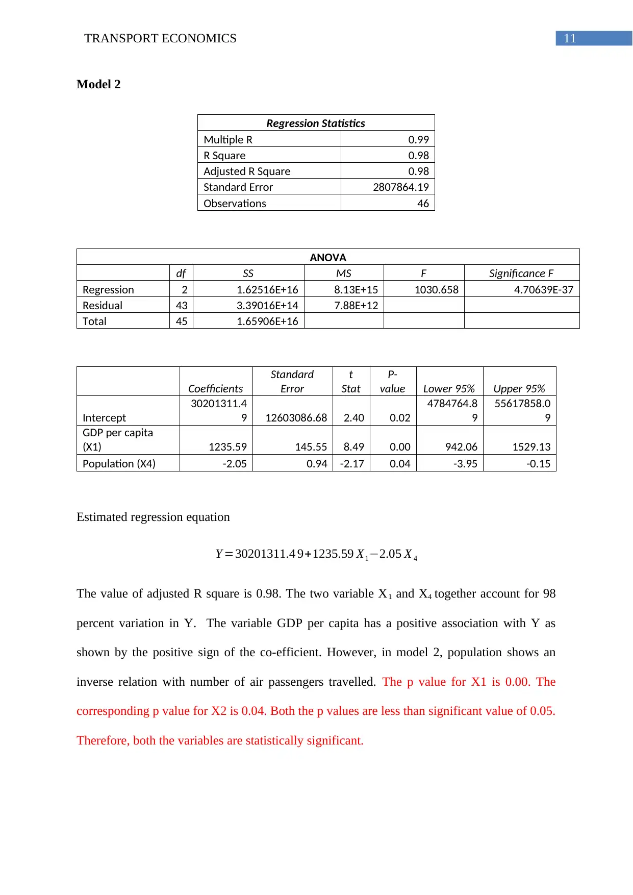
Model 2
Regression Statistics
Multiple R 0.99
R Square 0.98
Adjusted R Square 0.98
Standard Error 2807864.19
Observations 46
ANOVA
df SS MS F Significance F
Regression 2 1.62516E+16 8.13E+15 1030.658 4.70639E-37
Residual 43 3.39016E+14 7.88E+12
Total 45 1.65906E+16
Coefficients
Standard
Error
t
Stat
P-
value Lower 95% Upper 95%
Intercept
30201311.4
9 12603086.68 2.40 0.02
4784764.8
9
55617858.0
9
GDP per capita
(X1) 1235.59 145.55 8.49 0.00 942.06 1529.13
Population (X4) -2.05 0.94 -2.17 0.04 -3.95 -0.15
Estimated regression equation
Y =30201311.4 9+1235.59 X1−2.05 X 4
The value of adjusted R square is 0.98. The two variable X1 and X4 together account for 98
percent variation in Y. The variable GDP per capita has a positive association with Y as
shown by the positive sign of the co-efficient. However, in model 2, population shows an
inverse relation with number of air passengers travelled. The p value for X1 is 0.00. The
corresponding p value for X2 is 0.04. Both the p values are less than significant value of 0.05.
Therefore, both the variables are statistically significant.
⊘ This is a preview!⊘
Do you want full access?
Subscribe today to unlock all pages.
Trusted by 1+ million students worldwide
1 out of 17

Your All-in-One AI-Powered Toolkit for Academic Success.
+13062052269
info@desklib.com
Available 24*7 on WhatsApp / Email
![[object Object]](/_next/static/media/star-bottom.7253800d.svg)
Unlock your academic potential
Copyright © 2020–2026 A2Z Services. All Rights Reserved. Developed and managed by ZUCOL.