Macroeconomic Principles: Analysis of Economic Policies and Models

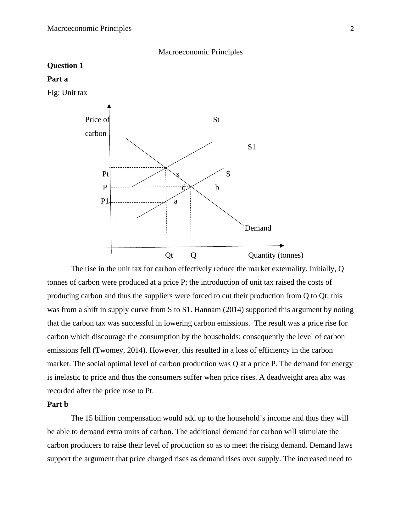
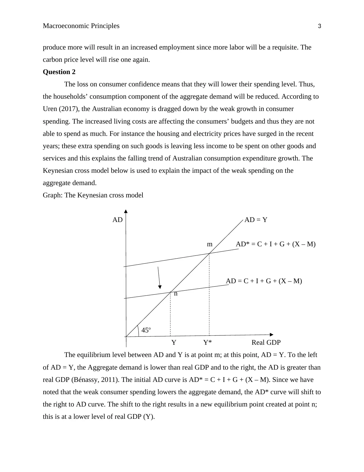
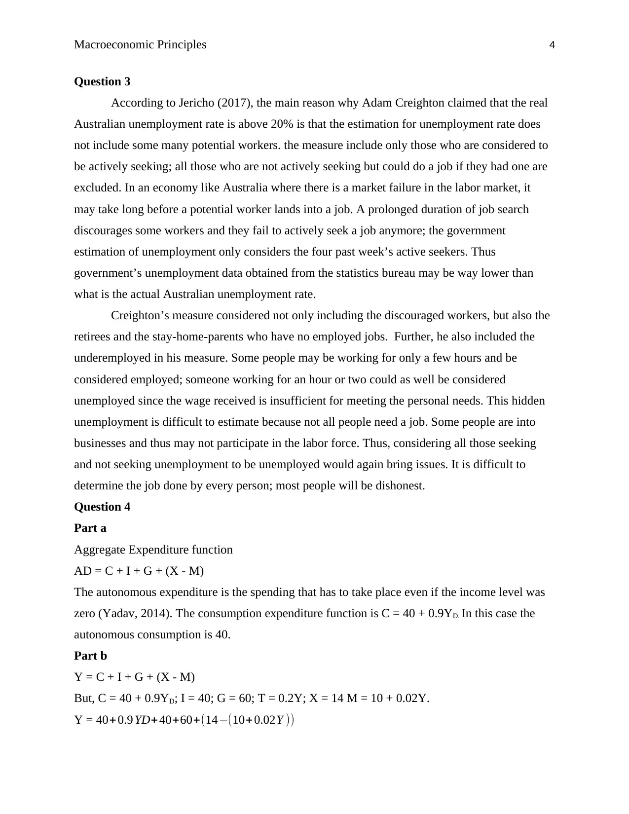
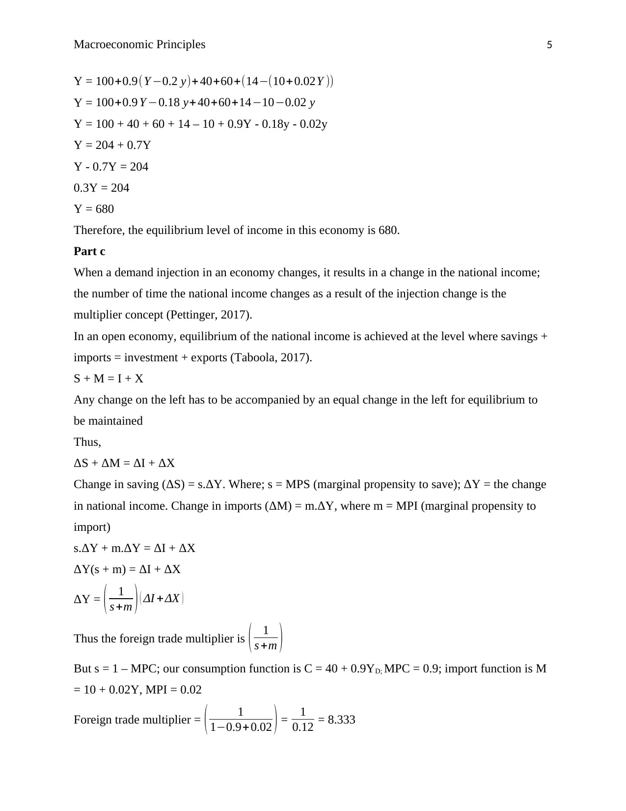
This assignment delves into key macroeconomic principles, analyzing the effects of a unit carbon tax on market externalities, the impact of declining consumer confidence on aggregate demand using the Keynesian cross model, and the complexities of measuring the Australian unemployment rate, including alternative perspectives on its estimation. Furthermore, it examines the aggregate expenditure function, calculating the equilibrium level of income and the foreign trade multiplier in an open economy. The assignment utilizes economic models and real-world examples to illustrate these concepts, supported by references to academic sources and news articles.

Running Head: Macroeconomic Principles
Macroeconomic Principles
By (Name)
(Tutor)
(University)
(Date)

Macroeconomic Principles 2
Macroeconomic Principles
Question 1
Part a
Fig: Unit tax
Price of St
carbon
S1
Pt x S
P d b
P1 a
Demand
Qt Q Quantity (tonnes)
The rise in the unit tax for carbon effectively reduce the market externality. Initially, Q
tonnes of carbon were produced at a price P; the introduction of unit tax raised the costs of
producing carbon and thus the suppliers were forced to cut their production from Q to Qt; this
was from a shift in supply curve from S to S1. Hannam (2014) supported this argument by noting
that the carbon tax was successful in lowering carbon emissions. The result was a price rise for
carbon which discourage the consumption by the households; consequently the level of carbon
emissions fell (Twomey, 2014). However, this resulted in a loss of efficiency in the carbon
market. The social optimal level of carbon production was Q at a price P. The demand for energy
is inelastic to price and thus the consumers suffer when price rises. A deadweight area abx was
recorded after the price rose to Pt.
Part b
The 15 billion compensation would add up to the household’s income and thus they will
be able to demand extra units of carbon. The additional demand for carbon will stimulate the
carbon producers to raise their level of production so as to meet the rising demand. Demand laws
support the argument that price charged rises as demand rises over supply. The increased need to

Macroeconomic Principles 3
produce more will result in an increased employment since more labor will be a requisite. The
carbon price level will rise one again.
Question 2
The loss on consumer confidence means that they will lower their spending level. Thus,
the households’ consumption component of the aggregate demand will be reduced. According to
Uren (2017), the Australian economy is dragged down by the weak growth in consumer
spending. The increased living costs are affecting the consumers’ budgets and thus they are not
able to spend as much. For instance the housing and electricity prices have surged in the recent
years; these extra spending on such goods is leaving less income to be spent on other goods and
services and this explains the falling trend of Australian consumption expenditure growth. The
Keynesian cross model below is used to explain the impact of the weak spending on the
aggregate demand.
Graph: The Keynesian cross model
AD AD = Y
m AD* = C + I + G + (X – M)
AD = C + I + G + (X – M)
n
45o
Y Y* Real GDP
The equilibrium level between AD and Y is at point m; at this point, AD = Y. To the left
of AD = Y, the Aggregate demand is lower than real GDP and to the right, the AD is greater than
real GDP (Bénassy, 2011). The initial AD curve is AD* = C + I + G + (X – M). Since we have
noted that the weak consumer spending lowers the aggregate demand, the AD* curve will shift to
the right to AD curve. The shift to the right results in a new equilibrium point created at point n;
this is at a lower level of real GDP (Y).

Macroeconomic Principles 4
Question 3
According to Jericho (2017), the main reason why Adam Creighton claimed that the real
Australian unemployment rate is above 20% is that the estimation for unemployment rate does
not include some many potential workers. the measure include only those who are considered to
be actively seeking; all those who are not actively seeking but could do a job if they had one are
excluded. In an economy like Australia where there is a market failure in the labor market, it
may take long before a potential worker lands into a job. A prolonged duration of job search
discourages some workers and they fail to actively seek a job anymore; the government
estimation of unemployment only considers the four past week’s active seekers. Thus
government’s unemployment data obtained from the statistics bureau may be way lower than
what is the actual Australian unemployment rate.
Creighton’s measure considered not only including the discouraged workers, but also the
retirees and the stay-home-parents who have no employed jobs. Further, he also included the
underemployed in his measure. Some people may be working for only a few hours and be
considered employed; someone working for an hour or two could as well be considered
unemployed since the wage received is insufficient for meeting the personal needs. This hidden
unemployment is difficult to estimate because not all people need a job. Some people are into
businesses and thus may not participate in the labor force. Thus, considering all those seeking
and not seeking unemployment to be unemployed would again bring issues. It is difficult to
determine the job done by every person; most people will be dishonest.
Question 4
Part a
Aggregate Expenditure function
AD = C + I + G + (X - M)
The autonomous expenditure is the spending that has to take place even if the income level was
zero (Yadav, 2014). The consumption expenditure function is C = 40 + 0.9YD. In this case the
autonomous consumption is 40.
Part b
Y = C + I + G + (X - M)
But, C = 40 + 0.9YD; I = 40; G = 60; T = 0.2Y; X = 14 M = 10 + 0.02Y.
Y = 40+ 0.9 YD+ 40+60+(14−(10+ 0.02Y ))

Macroeconomic Principles 5
Y = 100+0.9(Y −0.2 y)+ 40+60+(14−(10+0.02Y ))
Y = 100+0.9 Y −0.18 y+ 40+60+14−10−0.02 y
Y = 100 + 40 + 60 + 14 – 10 + 0.9Y - 0.18y - 0.02y
Y = 204 + 0.7Y
Y - 0.7Y = 204
0.3Y = 204
Y = 680
Therefore, the equilibrium level of income in this economy is 680.
Part c
When a demand injection in an economy changes, it results in a change in the national income;
the number of time the national income changes as a result of the injection change is the
multiplier concept (Pettinger, 2017).
In an open economy, equilibrium of the national income is achieved at the level where savings +
imports = investment + exports (Taboola, 2017).
S + M = I + X
Any change on the left has to be accompanied by an equal change in the left for equilibrium to
be maintained
Thus,
ΔS + ΔM = ΔI + ΔX
Change in saving (ΔS) = s.ΔY. Where; s = MPS (marginal propensity to save); ΔY = the change
in national income. Change in imports (ΔM) = m.ΔY, where m = MPI (marginal propensity to
import)
s.ΔY + m.ΔY = ΔI + ΔX
ΔY(s + m) = ΔI + ΔX
ΔY = ( 1
s +m ) ( ΔI +ΔX )
Thus the foreign trade multiplier is ( 1
s +m )
But s = 1 – MPC; our consumption function is C = 40 + 0.9YD; MPC = 0.9; import function is M
= 10 + 0.02Y, MPI = 0.02
Foreign trade multiplier = ( 1
1−0.9+ 0.02 ) = 1
0.12 = 8.333

Macroeconomic Principles 6
Multiplying 8.333 by the ∆ in exports (30-14 = 16) we get the change in national income
8.333*16 = 133.333
Change in national income = 133

Macroeconomic Principles 7
References
Bénassy, J. (2011). Macroeconomic theory. New York: Oxford University Press.
Hannam, P. (2014). Carbon price helped curb emissions, ANU study finds. [Online] The Sydney
Morning Herald. Available at: http://www.smh.com.au/environment/climate-change/carbon-
price-helped-curb-emissions-anu-study-finds-20140716-ztuf6.html [Accessed 2 Oct. 2017].
Jericho, G. (2017). To those who claim Australia's unemployment data is dishonest – please stop
| Greg Jericho. [Online] The Guardian. Available at:
https://www.theguardian.com/business/grogonomics/2017/may/30/to-those-who-claim-
australias-unemployment-data-is-dishonest-please-stop [Accessed 2 Oct. 2017].
Pettinger, T. (2017). The multiplier effect. [Online] Economicshelp.org. Available at:
https://www.economicshelp.org/blog/1948/economics/the-multiplier-effect/ [Accessed 2 Oct.
2017].
Taboola (2017). National Income and the Foreign Trade Multiplier. [Online] Economics
Discussion. Available at: http://www.economicsdiscussion.net/national-income/foreign-trade-
multiplier/national-income-and-the-foreign-trade-multiplier-2/10760 [Accessed 2 Oct. 2017].
Twomey, P. (2014). Obituary: Australia's carbon price. [Online] The Conversation. Available
at: https://theconversation.com/obituary-australias-carbon-price-29217 [Accessed 2 Oct. 2017].
Uren, D. (2017). Weak spend a drag on economy. [Online] Theaustralian.com.au. Available at:
http://www.theaustralian.com.au/business/opinion/david-uren-economics/weak-consumer-
spending-a-drag-on-economic-growth/news-story/5cf5c25bbdb6e119f5ca8517dfc40430
[Accessed 2 Oct. 2017].
Yadav, G. (2014). How are autonomous expenditures determined? [Online] Quora. Available at:
https://www.quora.com/How-are-autonomous-expenditures-determined [Accessed 2 Oct. 2017].