Statistics Assignment: Australian Exports, Regression, and Analysis

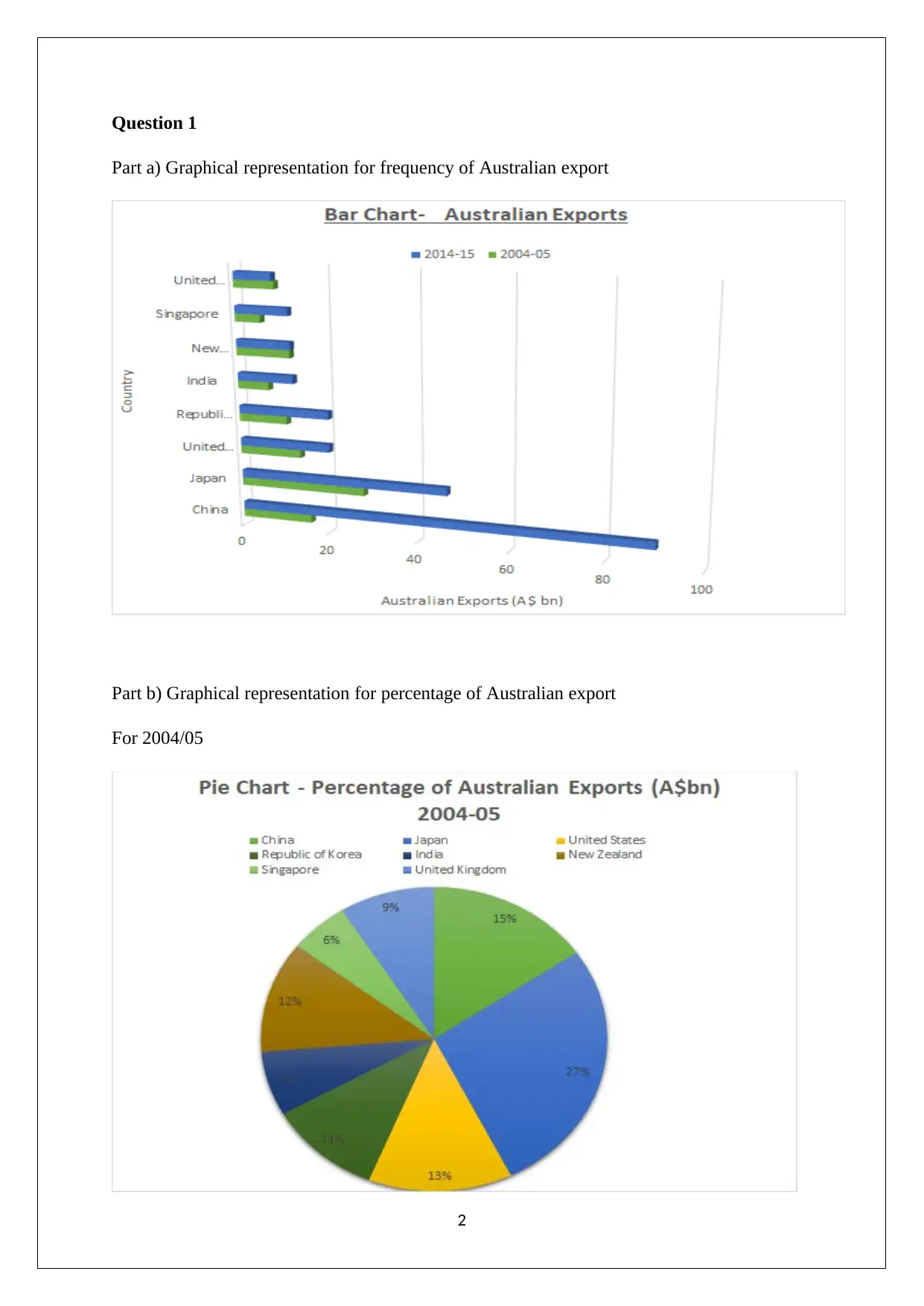
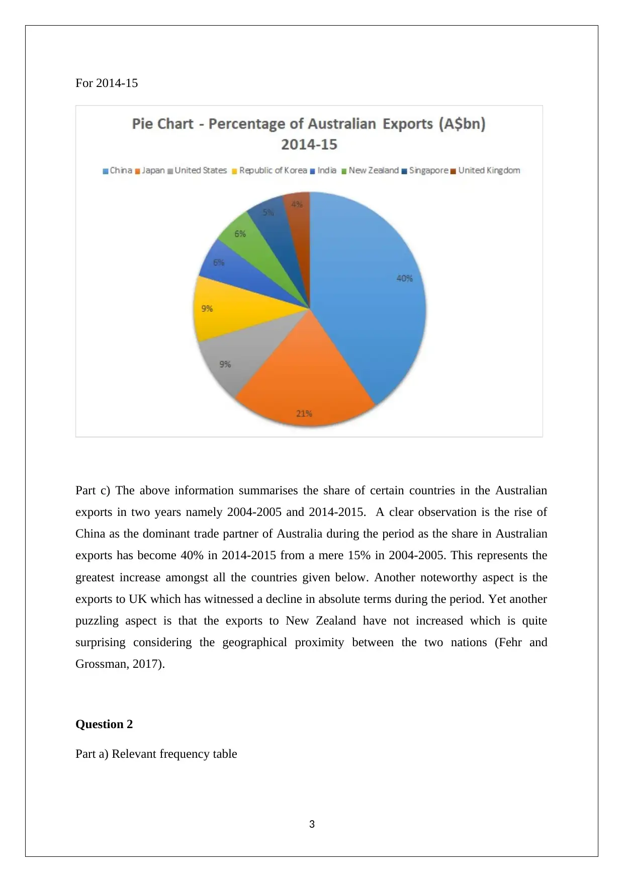
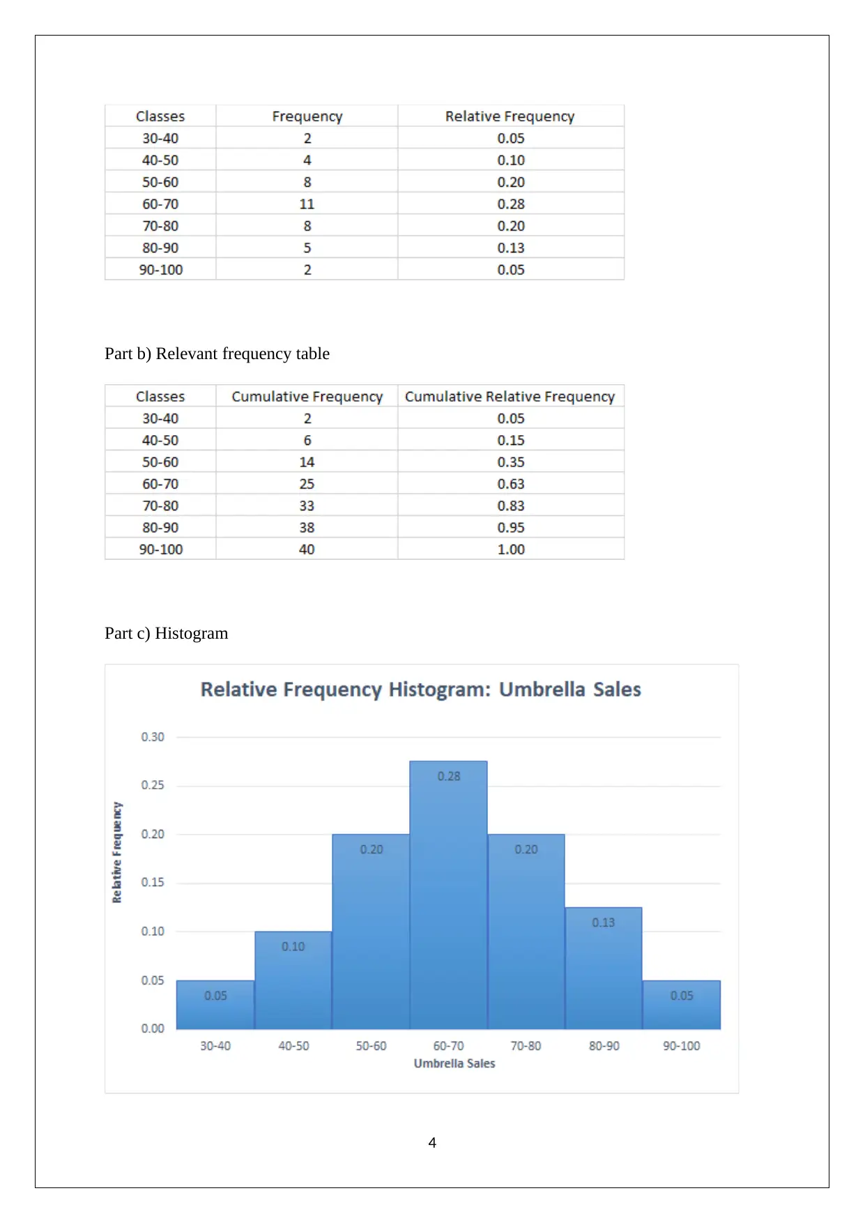
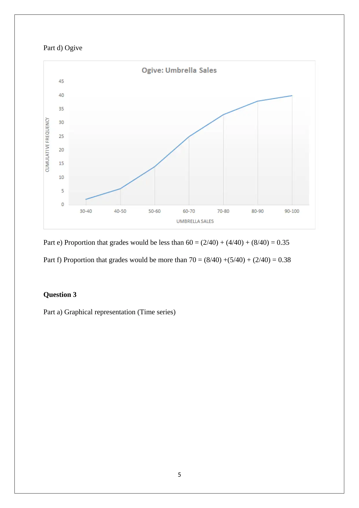
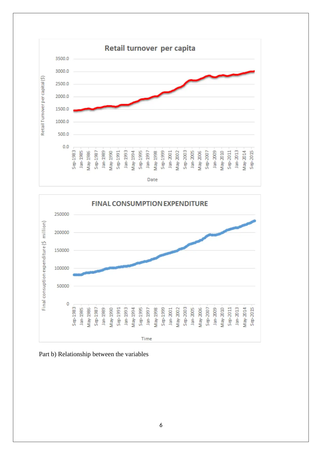
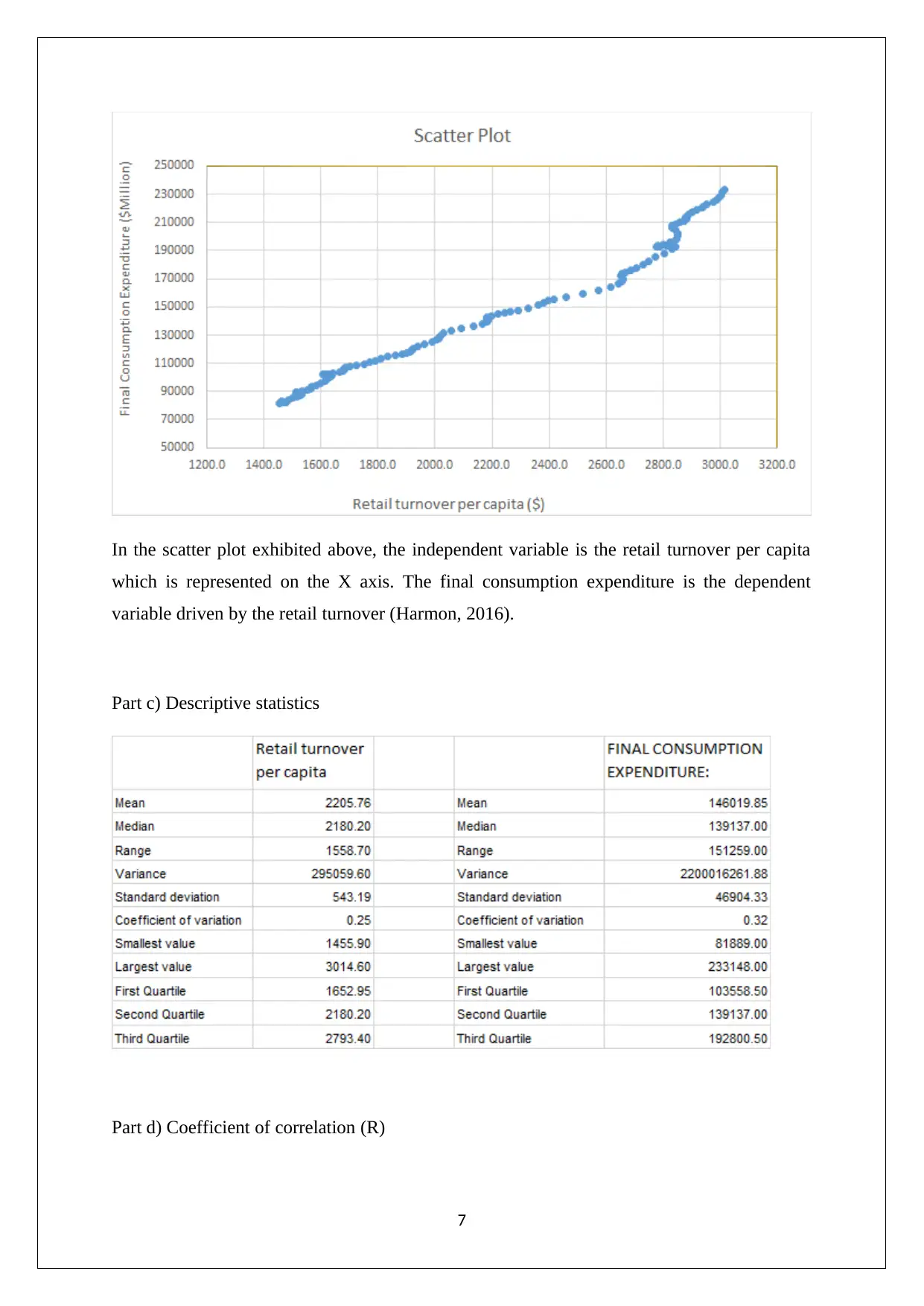
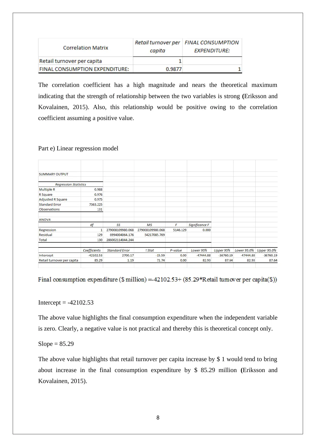
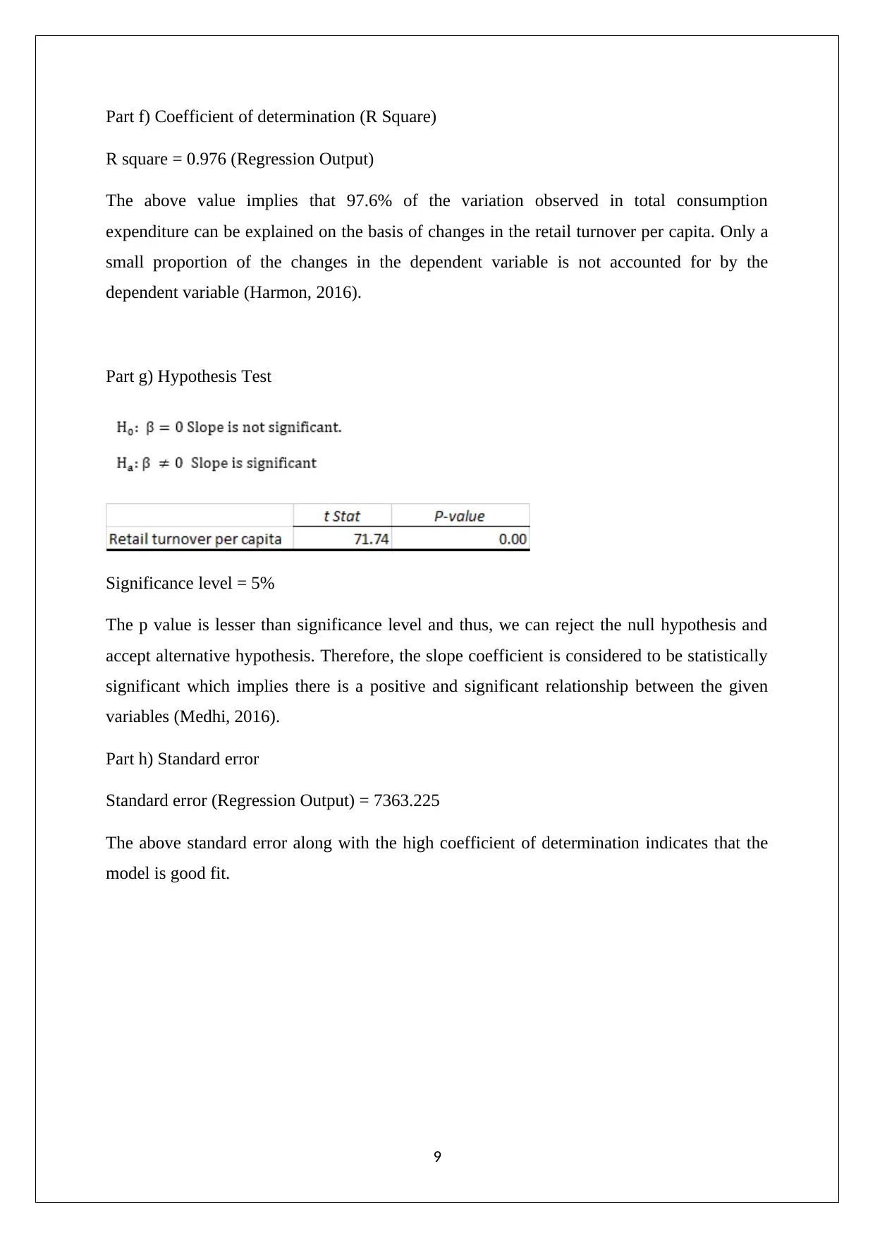
This statistics assignment analyzes Australian export data from 2004/05 and 2014-15, focusing on the changing trade relationships with countries like China and the UK. It includes graphical representations of frequency and percentage data, along with observations about the shifts in export partners. The assignment further delves into frequency tables, histograms, and ogives related to grades, calculating proportions based on these distributions. A time series analysis and scatter plot explore the relationship between retail turnover per capita and final consumption expenditure, including descriptive statistics, correlation coefficients, and a linear regression model. The analysis includes interpreting the intercept, slope, coefficient of determination, and conducting a hypothesis test to assess the statistical significance of the relationship between the variables. The assignment concludes with an evaluation of the model's fit using the standard error and includes a list of relevant academic references.

STATISTICS FOR BUSINESS DECISIONS
STUDENT ID:
[Pick the date]

Question 1
Part a) Graphical representation for frequency of Australian export
Part b) Graphical representation for percentage of Australian export
For 2004/05
2

For 2014-15
Part c) The above information summarises the share of certain countries in the Australian
exports in two years namely 2004-2005 and 2014-2015. A clear observation is the rise of
China as the dominant trade partner of Australia during the period as the share in Australian
exports has become 40% in 2014-2015 from a mere 15% in 2004-2005. This represents the
greatest increase amongst all the countries given below. Another noteworthy aspect is the
exports to UK which has witnessed a decline in absolute terms during the period. Yet another
puzzling aspect is that the exports to New Zealand have not increased which is quite
surprising considering the geographical proximity between the two nations (Fehr and
Grossman, 2017).
Question 2
Part a) Relevant frequency table
3

Part b) Relevant frequency table
Part c) Histogram
4

Part d) Ogive
Part e) Proportion that grades would be less than 60 = (2/40) + (4/40) + (8/40) = 0.35
Part f) Proportion that grades would be more than 70 = (8/40) +(5/40) + (2/40) = 0.38
Question 3
Part a) Graphical representation (Time series)
5

Part b) Relationship between the variables
6

In the scatter plot exhibited above, the independent variable is the retail turnover per capita
which is represented on the X axis. The final consumption expenditure is the dependent
variable driven by the retail turnover (Harmon, 2016).
Part c) Descriptive statistics
Part d) Coefficient of correlation (R)
7

The correlation coefficient has a high magnitude and nears the theoretical maximum
indicating that the strength of relationship between the two variables is strong (Eriksson and
Kovalainen, 2015). Also, this relationship would be positive owing to the correlation
coefficient assuming a positive value.
Part e) Linear regression model
Intercept = -42102.53
The above value highlights the final consumption expenditure when the independent variable
is zero. Clearly, a negative value is not practical and thereby this is theoretical concept only.
Slope = 85.29
The above value highlights that retail turnover per capita increase by $ 1 would tend to bring
about increase in the final consumption expenditure by $ 85.29 million (Eriksson and
Kovalainen, 2015).
8

Part f) Coefficient of determination (R Square)
R square = 0.976 (Regression Output)
The above value implies that 97.6% of the variation observed in total consumption
expenditure can be explained on the basis of changes in the retail turnover per capita. Only a
small proportion of the changes in the dependent variable is not accounted for by the
dependent variable (Harmon, 2016).
Part g) Hypothesis Test
Significance level = 5%
The p value is lesser than significance level and thus, we can reject the null hypothesis and
accept alternative hypothesis. Therefore, the slope coefficient is considered to be statistically
significant which implies there is a positive and significant relationship between the given
variables (Medhi, 2016).
Part h) Standard error
Standard error (Regression Output) = 7363.225
The above standard error along with the high coefficient of determination indicates that the
model is good fit.
9

References
Eriksson, P. and Kovalainen, A. (2015) Quantitative methods in business research. 3rd ed.
London: Sage Publications.
Fehr, F. H. and Grossman, G. (2017). An introduction to sets, probability and hypothesis
testing. 3rd ed. Ohio: Heath.
Harmon, M. (2016) Hypothesis Testing in Excel - The Excel Statistical Master. 7th ed.
Florida: Mark Harmon.
Medhi, J. (2016) Statistical Methods: An Introductory Text. 4th ed. Sydney: New Age
International.
10