Case Study: Gender Equality and Economic Impact in Australia
VerifiedAdded on 2021/06/15
|14
|2914
|302
Case Study
AI Summary
This case study investigates gender equality in Australia using datasets from the Australian Taxation Office (ATO) and the OECD. The research explores the relationship between gender, occupation, salary, and gifts/donations, utilizing descriptive and inferential statistics. Key findings reveal significant gender disparities in occupations and salaries, with males generally earning more. Inferential statistics, including hypothesis testing and regression analysis, confirm a statistically significant relationship between the gender wage gap and GDP. The study employs a regression model to analyze this relationship and suggests further research into the factors contributing to gender inequality and its economic consequences, emphasizing the importance of closing the gender gap for policy-making and economic development.
Running Header: Case Study on Gender equality in Australia 1
Case Study on Gender equality in Australia
Student’s name:
Student’s ID:
Institution:
Case Study on Gender equality in Australia
Student’s name:
Student’s ID:
Institution:
Paraphrase This Document
Need a fresh take? Get an instant paraphrase of this document with our AI Paraphraser
Case Study on Gender equality in Australia 2
Table of Contents
Section 1: Introduction................................................................................................................................3
1.b. Dataset 1 description........................................................................................................................4
1.c. Dataset 2 description........................................................................................................................5
Section 2: Descriptive Statistics...................................................................................................................6
2.a. The relationship between the Gender variable and Occupation......................................................6
2.b. The relationship between the Gender Variable and Salary or wage amount...................................6
2.c. The relationship between the variables Gender and Salary or wage amount (numerical summary)7
2.d. The relationship between the Salary or wage amount and gifts or donation deductions................8
Section 3: Inferential Statistics....................................................................................................................9
3.a Top 4 occupations based on median salary and proportion of the gender........................................9
3.b Significance of proportion of male machinery operators and drivers is more than 80%.................10
3.c Hypothesis test to determine whether there is a difference in salary amount between genders.. .11
3.d. Regression analysis (using dataset 2)..............................................................................................12
Section 4: Discussion & Conclusion...........................................................................................................13
4.a. Discussion and Conclusions of findings...........................................................................................13
4.b. Suggestions for further research....................................................................................................13
References.................................................................................................................................................14
Case Study on Gender equality in Australia 3
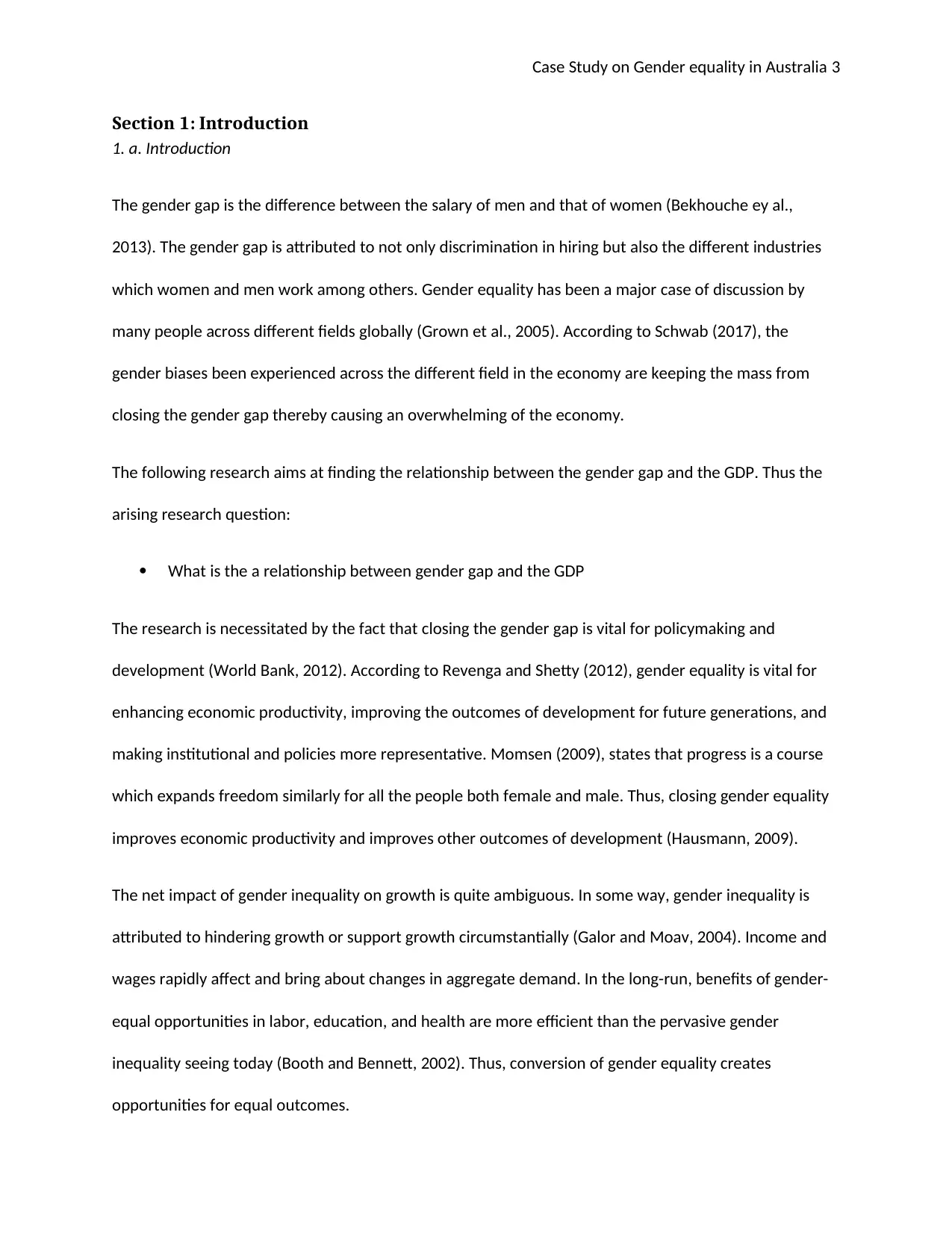
Section 1: Introduction
1. a. Introduction
The gender gap is the difference between the salary of men and that of women (Bekhouche ey al.,
2013). The gender gap is attributed to not only discrimination in hiring but also the different industries
which women and men work among others. Gender equality has been a major case of discussion by
many people across different fields globally (Grown et al., 2005). According to Schwab (2017), the
gender biases been experienced across the different field in the economy are keeping the mass from
closing the gender gap thereby causing an overwhelming of the economy.
The following research aims at finding the relationship between the gender gap and the GDP. Thus the
arising research question:
What is the a relationship between gender gap and the GDP
The research is necessitated by the fact that closing the gender gap is vital for policymaking and
development (World Bank, 2012). According to Revenga and Shetty (2012), gender equality is vital for
enhancing economic productivity, improving the outcomes of development for future generations, and
making institutional and policies more representative. Momsen (2009), states that progress is a course
which expands freedom similarly for all the people both female and male. Thus, closing gender equality
improves economic productivity and improves other outcomes of development (Hausmann, 2009).
The net impact of gender inequality on growth is quite ambiguous. In some way, gender inequality is
attributed to hindering growth or support growth circumstantially (Galor and Moav, 2004). Income and
wages rapidly affect and bring about changes in aggregate demand. In the long-run, benefits of gender-
equal opportunities in labor, education, and health are more efficient than the pervasive gender
inequality seeing today (Booth and Bennett, 2002). Thus, conversion of gender equality creates
opportunities for equal outcomes.
⊘ This is a preview!⊘
Do you want full access?
Subscribe today to unlock all pages.
Trusted by 1+ million students worldwide
Case Study on Gender equality in Australia 4
Therefore, the question that arises is whether differences in wages and income affect economic growth
or not? The following research will, therefore, endeavor to determine whether gender inequality has an
economic impact. Thus, this provides a guide for the researcher to determine if indeed there is a
relationship between gender gap and the GDP.
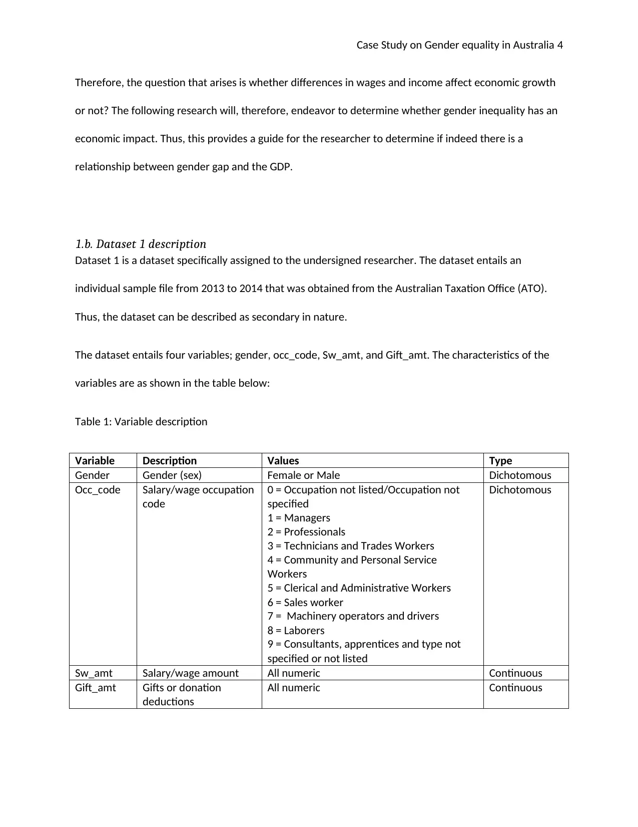
1.b. Dataset 1 description
Dataset 1 is a dataset specifically assigned to the undersigned researcher. The dataset entails an
individual sample file from 2013 to 2014 that was obtained from the Australian Taxation Office (ATO).
Thus, the dataset can be described as secondary in nature.
The dataset entails four variables; gender, occ_code, Sw_amt, and Gift_amt. The characteristics of the
variables are as shown in the table below:
Table 1: Variable description
Variable Description Values Type
Gender Gender (sex) Female or Male Dichotomous
Occ_code Salary/wage occupation
code
0 = Occupation not listed/Occupation not
specified
1 = Managers
2 = Professionals
3 = Technicians and Trades Workers
4 = Community and Personal Service
Workers
5 = Clerical and Administrative Workers
6 = Sales worker
7 = Machinery operators and drivers
8 = Laborers
9 = Consultants, apprentices and type not
specified or not listed
Dichotomous
Sw_amt Salary/wage amount All numeric Continuous
Gift_amt Gifts or donation
deductions
All numeric Continuous
Therefore, the question that arises is whether differences in wages and income affect economic growth
or not? The following research will, therefore, endeavor to determine whether gender inequality has an
economic impact. Thus, this provides a guide for the researcher to determine if indeed there is a
relationship between gender gap and the GDP.
1.b. Dataset 1 description
Dataset 1 is a dataset specifically assigned to the undersigned researcher. The dataset entails an
individual sample file from 2013 to 2014 that was obtained from the Australian Taxation Office (ATO).
Thus, the dataset can be described as secondary in nature.
The dataset entails four variables; gender, occ_code, Sw_amt, and Gift_amt. The characteristics of the
variables are as shown in the table below:
Table 1: Variable description
Variable Description Values Type
Gender Gender (sex) Female or Male Dichotomous
Occ_code Salary/wage occupation
code
0 = Occupation not listed/Occupation not
specified
1 = Managers
2 = Professionals
3 = Technicians and Trades Workers
4 = Community and Personal Service
Workers
5 = Clerical and Administrative Workers
6 = Sales worker
7 = Machinery operators and drivers
8 = Laborers
9 = Consultants, apprentices and type not
specified or not listed
Dichotomous
Sw_amt Salary/wage amount All numeric Continuous
Gift_amt Gifts or donation
deductions
All numeric Continuous
Paraphrase This Document
Need a fresh take? Get an instant paraphrase of this document with our AI Paraphraser
Case Study on Gender equality in Australia 5
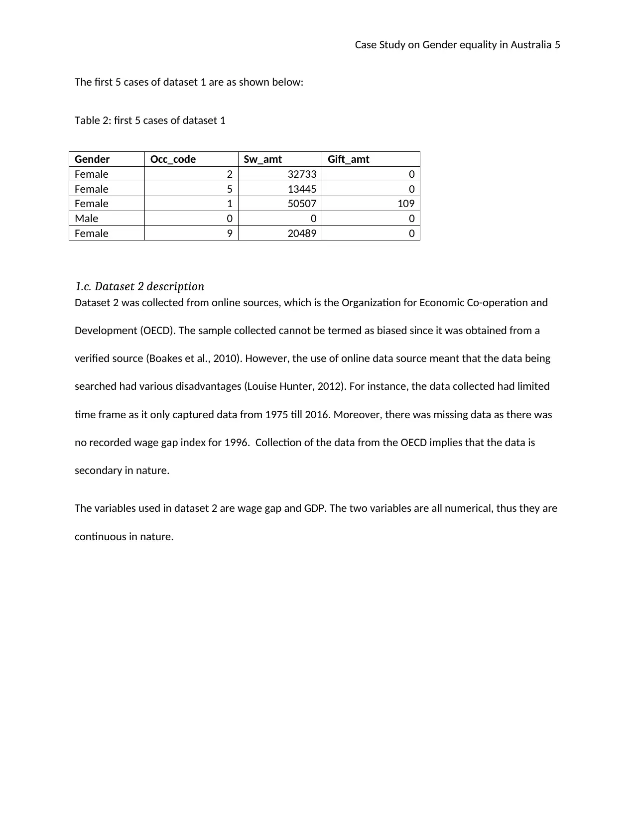
The first 5 cases of dataset 1 are as shown below:
Table 2: first 5 cases of dataset 1
Gender Occ_code Sw_amt Gift_amt
Female 2 32733 0
Female 5 13445 0
Female 1 50507 109
Male 0 0 0
Female 9 20489 0
1.c. Dataset 2 description
Dataset 2 was collected from online sources, which is the Organization for Economic Co-operation and
Development (OECD). The sample collected cannot be termed as biased since it was obtained from a
verified source (Boakes et al., 2010). However, the use of online data source meant that the data being
searched had various disadvantages (Louise Hunter, 2012). For instance, the data collected had limited
time frame as it only captured data from 1975 till 2016. Moreover, there was missing data as there was
no recorded wage gap index for 1996. Collection of the data from the OECD implies that the data is
secondary in nature.
The variables used in dataset 2 are wage gap and GDP. The two variables are all numerical, thus they are
continuous in nature.
Case Study on Gender equality in Australia 6
Section 2: Descriptive Statistics
2.a. The relationship between the Gender variable and Occupation
The relationship between the gender variable and occupation can is as seen in the figure below:
0 1 2 3 4 5 6 7 8 9
46% 42%
52%
12%
64%
72%
65%
6%
30%
45%
54% 58%
48%
88%
36%
28%
35%
94%
70%
55%
Gender Distribution against Occupation
% Female % Male
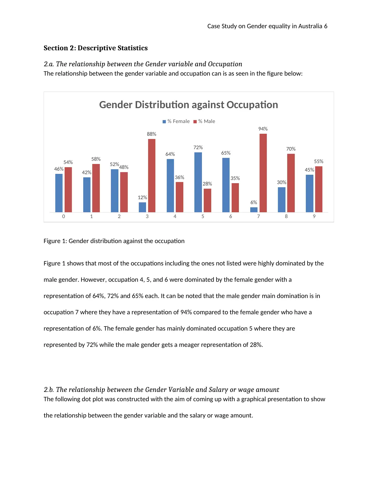
Figure 1: Gender distribution against the occupation
Figure 1 shows that most of the occupations including the ones not listed were highly dominated by the
male gender. However, occupation 4, 5, and 6 were dominated by the female gender with a
representation of 64%, 72% and 65% each. It can be noted that the male gender main domination is in
occupation 7 where they have a representation of 94% compared to the female gender who have a
representation of 6%. The female gender has mainly dominated occupation 5 where they are
represented by 72% while the male gender gets a meager representation of 28%.
2.b. The relationship between the Gender Variable and Salary or wage amount
The following dot plot was constructed with the aim of coming up with a graphical presentation to show
the relationship between the gender variable and the salary or wage amount.
Section 2: Descriptive Statistics
2.a. The relationship between the Gender variable and Occupation
The relationship between the gender variable and occupation can is as seen in the figure below:
0 1 2 3 4 5 6 7 8 9
46% 42%
52%
12%
64%
72%
65%
6%
30%
45%
54% 58%
48%
88%
36%
28%
35%
94%
70%
55%
Gender Distribution against Occupation
% Female % Male
Figure 1: Gender distribution against the occupation
Figure 1 shows that most of the occupations including the ones not listed were highly dominated by the
male gender. However, occupation 4, 5, and 6 were dominated by the female gender with a
representation of 64%, 72% and 65% each. It can be noted that the male gender main domination is in
occupation 7 where they have a representation of 94% compared to the female gender who have a
representation of 6%. The female gender has mainly dominated occupation 5 where they are
represented by 72% while the male gender gets a meager representation of 28%.
2.b. The relationship between the Gender Variable and Salary or wage amount
The following dot plot was constructed with the aim of coming up with a graphical presentation to show
the relationship between the gender variable and the salary or wage amount.
⊘ This is a preview!⊘
Do you want full access?
Subscribe today to unlock all pages.
Trusted by 1+ million students worldwide
Case Study on Gender equality in Australia 7
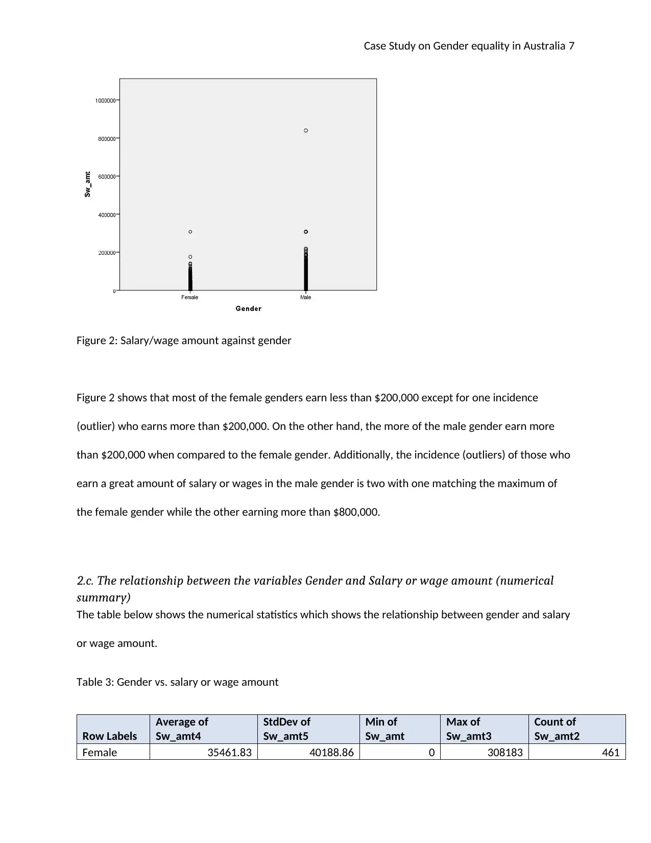
Figure 2: Salary/wage amount against gender
Figure 2 shows that most of the female genders earn less than $200,000 except for one incidence
(outlier) who earns more than $200,000. On the other hand, the more of the male gender earn more
than $200,000 when compared to the female gender. Additionally, the incidence (outliers) of those who
earn a great amount of salary or wages in the male gender is two with one matching the maximum of
the female gender while the other earning more than $800,000.
2.c. The relationship between the variables Gender and Salary or wage amount (numerical
summary)
The table below shows the numerical statistics which shows the relationship between gender and salary
or wage amount.
Table 3: Gender vs. salary or wage amount
Row Labels
Average of
Sw_amt4
StdDev of
Sw_amt5
Min of
Sw_amt
Max of
Sw_amt3
Count of
Sw_amt2
Female 35461.83 40188.86 0 308183 461
Paraphrase This Document
Need a fresh take? Get an instant paraphrase of this document with our AI Paraphraser
Case Study on Gender equality in Australia 8
Male 55679.90 68244.44 0 839840 539
Grand Total 46359.37 57909.58 0 839840 1000
The mean of female gender with regards to salary or wage amount is $35461.83 with a standard
deviation of $40,188.86. On the other hand, the male gender had a salary or wage amount that
averaged $55,679.90 with a standard deviation of $68,244.44. From this, it is evident that the male
gender earned a high salary or wage amount compared with the female gender. Conversely, the male
gender had a high variation ($8,244.44 standard deviation) compared to the female gender ($40,188.86
standard deviation).
2.d. The relationship between the Salary or wage amount and gifts or donation deductions
0
100000
200000
300000
400000
500000
600000
700000
800000
900000
0
1000
2000
3000
4000
5000
6000
7000
8000
9000
10000
Salary/wage amount Vs. Gifts or donation
deductions
Gift_amt
Linear (Gift_amt)
Sw_amt
Gft_amt
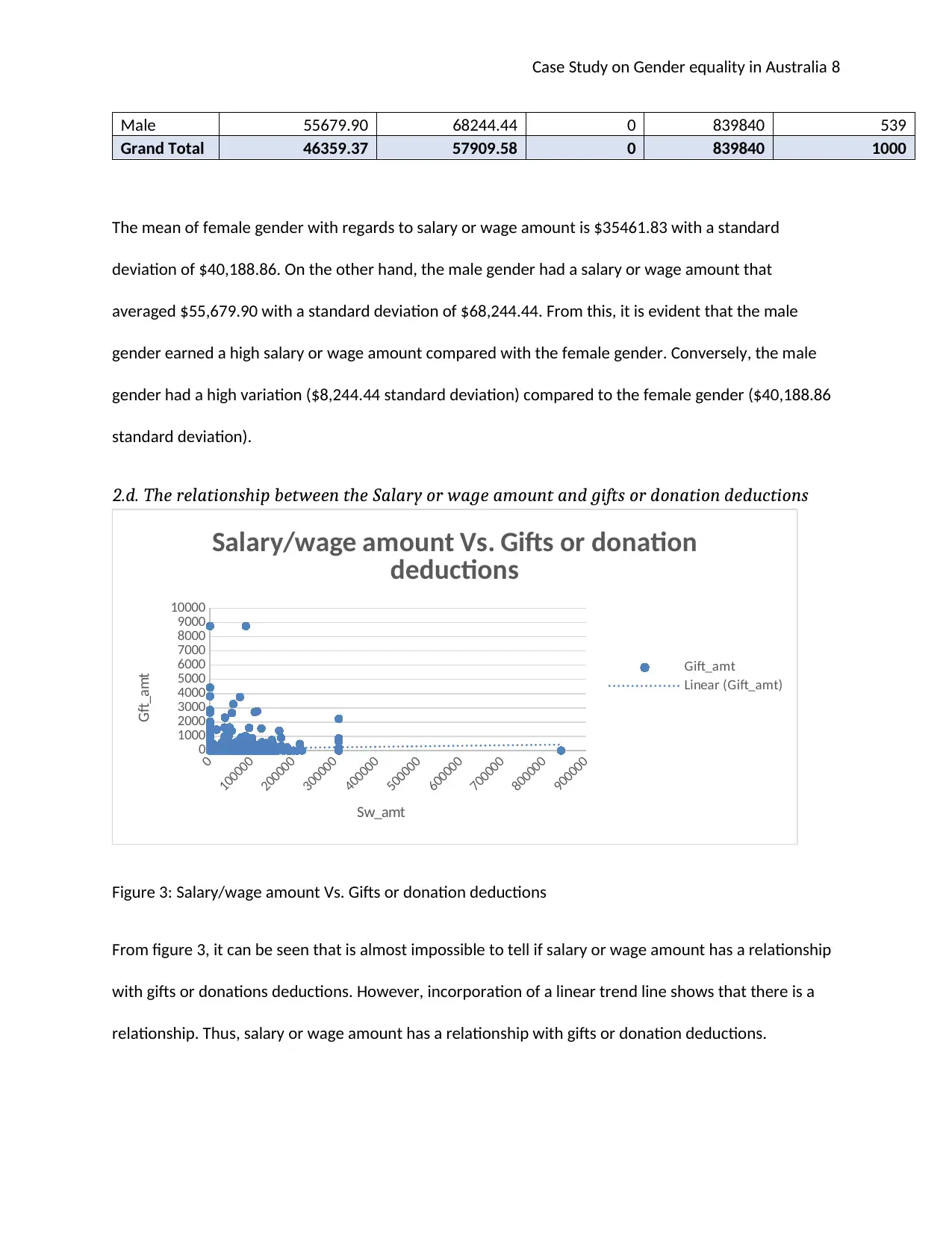
Figure 3: Salary/wage amount Vs. Gifts or donation deductions
From figure 3, it can be seen that is almost impossible to tell if salary or wage amount has a relationship
with gifts or donations deductions. However, incorporation of a linear trend line shows that there is a
relationship. Thus, salary or wage amount has a relationship with gifts or donation deductions.
Male 55679.90 68244.44 0 839840 539
Grand Total 46359.37 57909.58 0 839840 1000
The mean of female gender with regards to salary or wage amount is $35461.83 with a standard
deviation of $40,188.86. On the other hand, the male gender had a salary or wage amount that
averaged $55,679.90 with a standard deviation of $68,244.44. From this, it is evident that the male
gender earned a high salary or wage amount compared with the female gender. Conversely, the male
gender had a high variation ($8,244.44 standard deviation) compared to the female gender ($40,188.86
standard deviation).
2.d. The relationship between the Salary or wage amount and gifts or donation deductions
0
100000
200000
300000
400000
500000
600000
700000
800000
900000
0
1000
2000
3000
4000
5000
6000
7000
8000
9000
10000
Salary/wage amount Vs. Gifts or donation
deductions
Gift_amt
Linear (Gift_amt)
Sw_amt
Gft_amt
Figure 3: Salary/wage amount Vs. Gifts or donation deductions
From figure 3, it can be seen that is almost impossible to tell if salary or wage amount has a relationship
with gifts or donations deductions. However, incorporation of a linear trend line shows that there is a
relationship. Thus, salary or wage amount has a relationship with gifts or donation deductions.
Case Study on Gender equality in Australia 9
Section 3: Inferential Statistics
Use Dataset 1
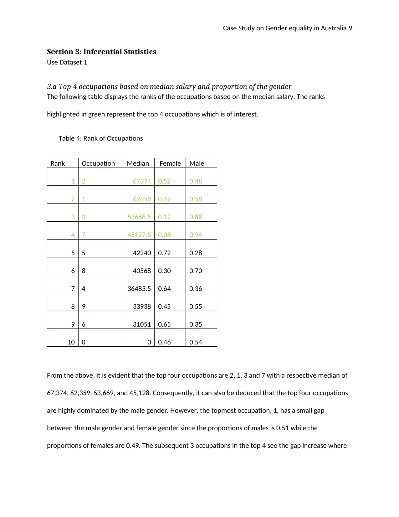
3.a Top 4 occupations based on median salary and proportion of the gender
The following table displays the ranks of the occupations based on the median salary. The ranks
highlighted in green represent the top 4 occupations which is of interest.
Table 4: Rank of Occupations
Rank Occupation Median Female Male
1 2 67374 0.52 0.48
2 1 62359 0.42 0.58
3 3 53668.5 0.12 0.88
4 7 45127.5 0.06 0.94
5 5 42240 0.72 0.28
6 8 40568 0.30 0.70
7 4 36485.5 0.64 0.36
8 9 33938 0.45 0.55
9 6 31051 0.65 0.35
10 0 0 0.46 0.54
From the above, it is evident that the top four occupations are 2, 1, 3 and 7 with a respective median of
67,374, 62,359, 53,669, and 45,128. Consequently, it can also be deduced that the top four occupations
are highly dominated by the male gender. However, the topmost occupation, 1, has a small gap
between the male gender and female gender since the proportions of males is 0.51 while the
proportions of females are 0.49. The subsequent 3 occupations in the top 4 see the gap increase where
Section 3: Inferential Statistics
Use Dataset 1
3.a Top 4 occupations based on median salary and proportion of the gender
The following table displays the ranks of the occupations based on the median salary. The ranks
highlighted in green represent the top 4 occupations which is of interest.
Table 4: Rank of Occupations
Rank Occupation Median Female Male
1 2 67374 0.52 0.48
2 1 62359 0.42 0.58
3 3 53668.5 0.12 0.88
4 7 45127.5 0.06 0.94
5 5 42240 0.72 0.28
6 8 40568 0.30 0.70
7 4 36485.5 0.64 0.36
8 9 33938 0.45 0.55
9 6 31051 0.65 0.35
10 0 0 0.46 0.54
From the above, it is evident that the top four occupations are 2, 1, 3 and 7 with a respective median of
67,374, 62,359, 53,669, and 45,128. Consequently, it can also be deduced that the top four occupations
are highly dominated by the male gender. However, the topmost occupation, 1, has a small gap
between the male gender and female gender since the proportions of males is 0.51 while the
proportions of females are 0.49. The subsequent 3 occupations in the top 4 see the gap increase where
⊘ This is a preview!⊘
Do you want full access?
Subscribe today to unlock all pages.
Trusted by 1+ million students worldwide
Case Study on Gender equality in Australia 10
1 has a difference of 0.22, 3 has a difference of 0.68 and 7 has a difference of 0.86 in the gender
proportions.
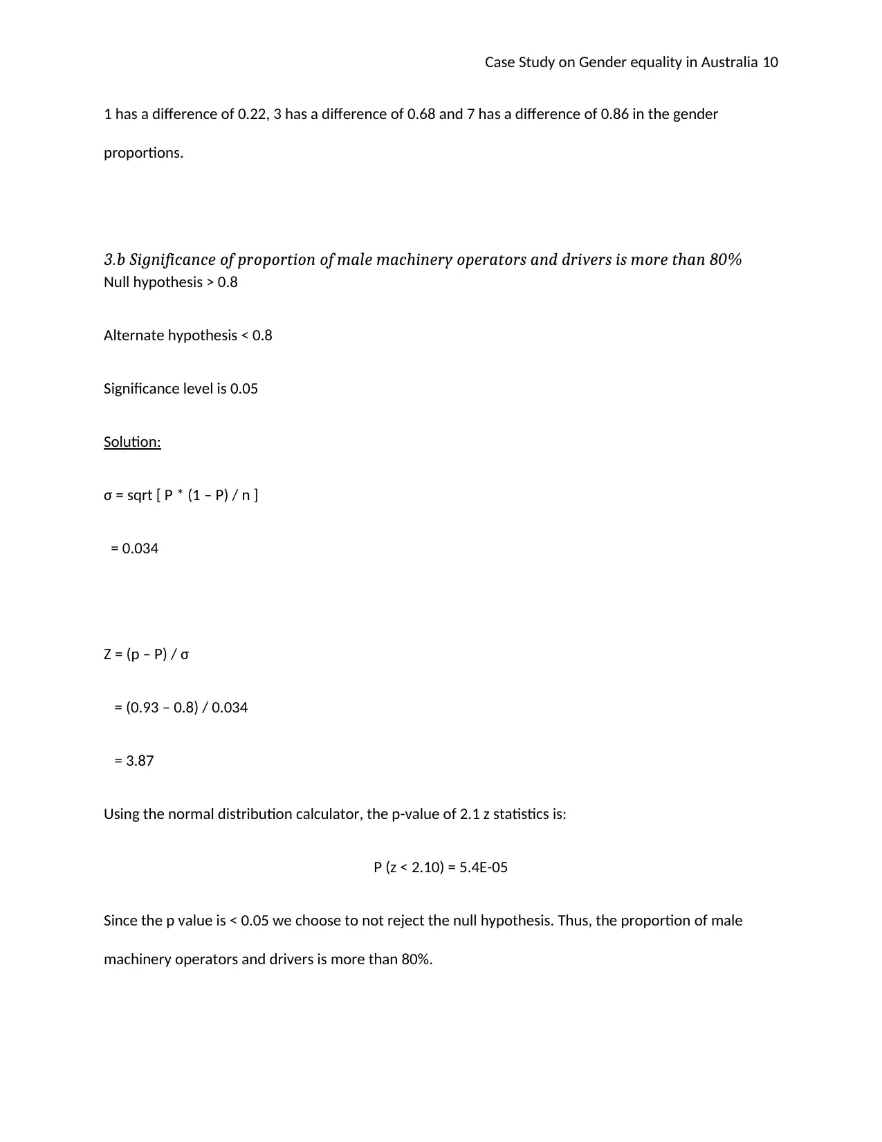
3.b Significance of proportion of male machinery operators and drivers is more than 80%
Null hypothesis > 0.8
Alternate hypothesis < 0.8
Significance level is 0.05
Solution:
σ = sqrt [ P * (1 – P) / n ]
= 0.034
Z = (p – P) / σ
= (0.93 – 0.8) / 0.034
= 3.87
Using the normal distribution calculator, the p-value of 2.1 z statistics is:
P (z < 2.10) = 5.4E-05
Since the p value is < 0.05 we choose to not reject the null hypothesis. Thus, the proportion of male
machinery operators and drivers is more than 80%.
1 has a difference of 0.22, 3 has a difference of 0.68 and 7 has a difference of 0.86 in the gender
proportions.
3.b Significance of proportion of male machinery operators and drivers is more than 80%
Null hypothesis > 0.8
Alternate hypothesis < 0.8
Significance level is 0.05
Solution:
σ = sqrt [ P * (1 – P) / n ]
= 0.034
Z = (p – P) / σ
= (0.93 – 0.8) / 0.034
= 3.87
Using the normal distribution calculator, the p-value of 2.1 z statistics is:
P (z < 2.10) = 5.4E-05
Since the p value is < 0.05 we choose to not reject the null hypothesis. Thus, the proportion of male
machinery operators and drivers is more than 80%.
Paraphrase This Document
Need a fresh take? Get an instant paraphrase of this document with our AI Paraphraser
Case Study on Gender equality in Australia 11
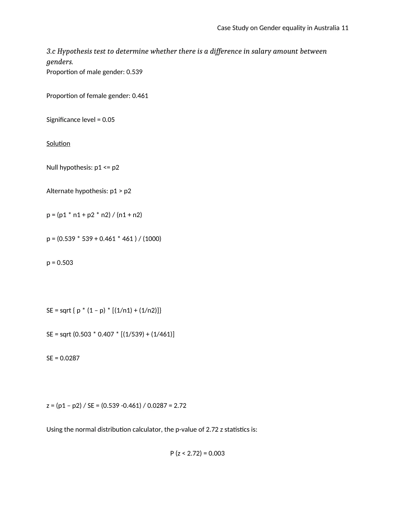
3.c Hypothesis test to determine whether there is a difference in salary amount between
genders.
Proportion of male gender: 0.539
Proportion of female gender: 0.461
Significance level = 0.05
Solution
Null hypothesis: p1 <= p2
Alternate hypothesis: p1 > p2
p = (p1 * n1 + p2 * n2) / (n1 + n2)
p = (0.539 * 539 + 0.461 * 461 ) / (1000)
p = 0.503
SE = sqrt { p * (1 – p) * [(1/n1) + (1/n2)]}
SE = sqrt (0.503 * 0.407 * [(1/539) + (1/461)]
SE = 0.0287
z = (p1 – p2) / SE = (0.539 -0.461) / 0.0287 = 2.72
Using the normal distribution calculator, the p-value of 2.72 z statistics is:
P (z < 2.72) = 0.003
Case Study on Gender equality in Australia 12
Since the p value is < 0.05 we choose to reject the null hypothesis (Higgins et al., 2003). Thus, the
proportion of the male gender is more than that of the female gender.
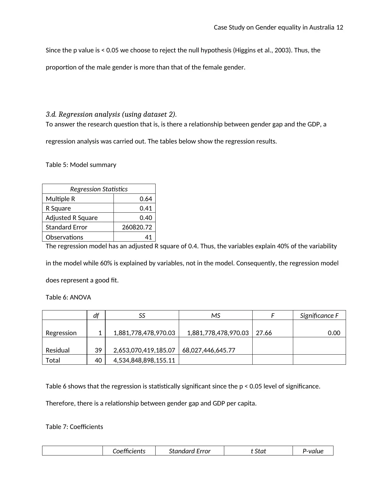
3.d. Regression analysis (using dataset 2).
To answer the research question that is, is there a relationship between gender gap and the GDP, a
regression analysis was carried out. The tables below show the regression results.
Table 5: Model summary
Regression Statistics
Multiple R 0.64
R Square 0.41
Adjusted R Square 0.40
Standard Error 260820.72
Observations 41
The regression model has an adjusted R square of 0.4. Thus, the variables explain 40% of the variability
in the model while 60% is explained by variables, not in the model. Consequently, the regression model
does represent a good fit.
Table 6: ANOVA
df SS MS F Significance F
Regression 1 1,881,778,478,970.03 1,881,778,478,970.03 27.66 0.00
Residual 39 2,653,070,419,185.07 68,027,446,645.77
Total 40 4,534,848,898,155.11
Table 6 shows that the regression is statistically significant since the p < 0.05 level of significance.
Therefore, there is a relationship between gender gap and GDP per capita.
Table 7: Coefficients
Coefficients Standard Error t Stat P-value
Since the p value is < 0.05 we choose to reject the null hypothesis (Higgins et al., 2003). Thus, the
proportion of the male gender is more than that of the female gender.
3.d. Regression analysis (using dataset 2).
To answer the research question that is, is there a relationship between gender gap and the GDP, a
regression analysis was carried out. The tables below show the regression results.
Table 5: Model summary
Regression Statistics
Multiple R 0.64
R Square 0.41
Adjusted R Square 0.40
Standard Error 260820.72
Observations 41
The regression model has an adjusted R square of 0.4. Thus, the variables explain 40% of the variability
in the model while 60% is explained by variables, not in the model. Consequently, the regression model
does represent a good fit.
Table 6: ANOVA
df SS MS F Significance F
Regression 1 1,881,778,478,970.03 1,881,778,478,970.03 27.66 0.00
Residual 39 2,653,070,419,185.07 68,027,446,645.77
Total 40 4,534,848,898,155.11
Table 6 shows that the regression is statistically significant since the p < 0.05 level of significance.
Therefore, there is a relationship between gender gap and GDP per capita.
Table 7: Coefficients
Coefficients Standard Error t Stat P-value
⊘ This is a preview!⊘
Do you want full access?
Subscribe today to unlock all pages.
Trusted by 1+ million students worldwide
1 out of 14
Related Documents


Your All-in-One AI-Powered Toolkit for Academic Success.
+13062052269
info@desklib.com
Available 24*7 on WhatsApp / Email
![[object Object]](/_next/static/media/star-bottom.7253800d.svg)
Unlock your academic potential
Copyright © 2020–2026 A2Z Services. All Rights Reserved. Developed and managed by ZUCOL.