Quantitative Methods Report: Student Environmental Perception Analysis
VerifiedAdded on 2020/03/28
|13
|2182
|277
Report
AI Summary
This report presents a quantitative analysis of student demographics and environmental perceptions in Australia. The study examines the gender distribution, height, and family time of students in VIC and NSW, utilizing both nominal and ratio scale data. Descriptive statistics, including averages and standard deviations, are computed to provide insights into the sample characteristics. The report explores students' attitudes towards environmental conservation, such as installing water tanks and powering off main switches. Furthermore, the study employs linear regression models to assess the relationship between hours spent in paid work and weekly income. The findings reveal differences in gender distributions, height, and family time between the two states. The regression analysis indicates no significant association between work hours and income. The report concludes with recommendations for promoting environmental awareness among students. The analysis was performed using Excel Spreadsheet, and the data was analyzed to understand the characteristics of the population and the relationship between the variables.
Running head: QUANTITATIVE METHODS
Quantitative Methods
Name:
Institution:
Quantitative Methods
Name:
Institution:
Paraphrase This Document
Need a fresh take? Get an instant paraphrase of this document with our AI Paraphraser
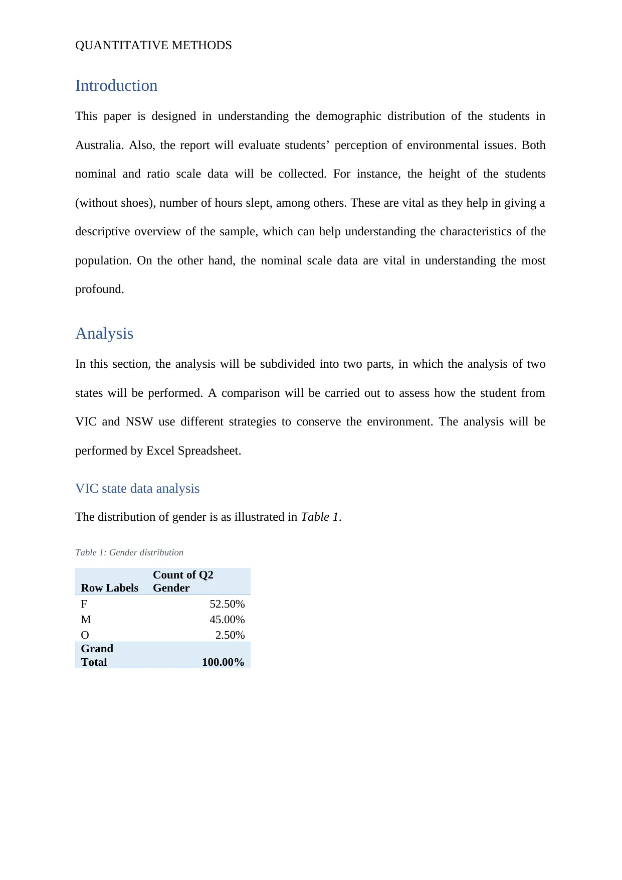
QUANTITATIVE METHODS
Introduction
This paper is designed in understanding the demographic distribution of the students in
Australia. Also, the report will evaluate students’ perception of environmental issues. Both
nominal and ratio scale data will be collected. For instance, the height of the students
(without shoes), number of hours slept, among others. These are vital as they help in giving a
descriptive overview of the sample, which can help understanding the characteristics of the
population. On the other hand, the nominal scale data are vital in understanding the most
profound.
Analysis
In this section, the analysis will be subdivided into two parts, in which the analysis of two
states will be performed. A comparison will be carried out to assess how the student from
VIC and NSW use different strategies to conserve the environment. The analysis will be
performed by Excel Spreadsheet.
VIC state data analysis
The distribution of gender is as illustrated in Table 1.
Table 1: Gender distribution
Row Labels
Count of Q2
Gender
F 52.50%
M 45.00%
O 2.50%
Grand
Total 100.00%
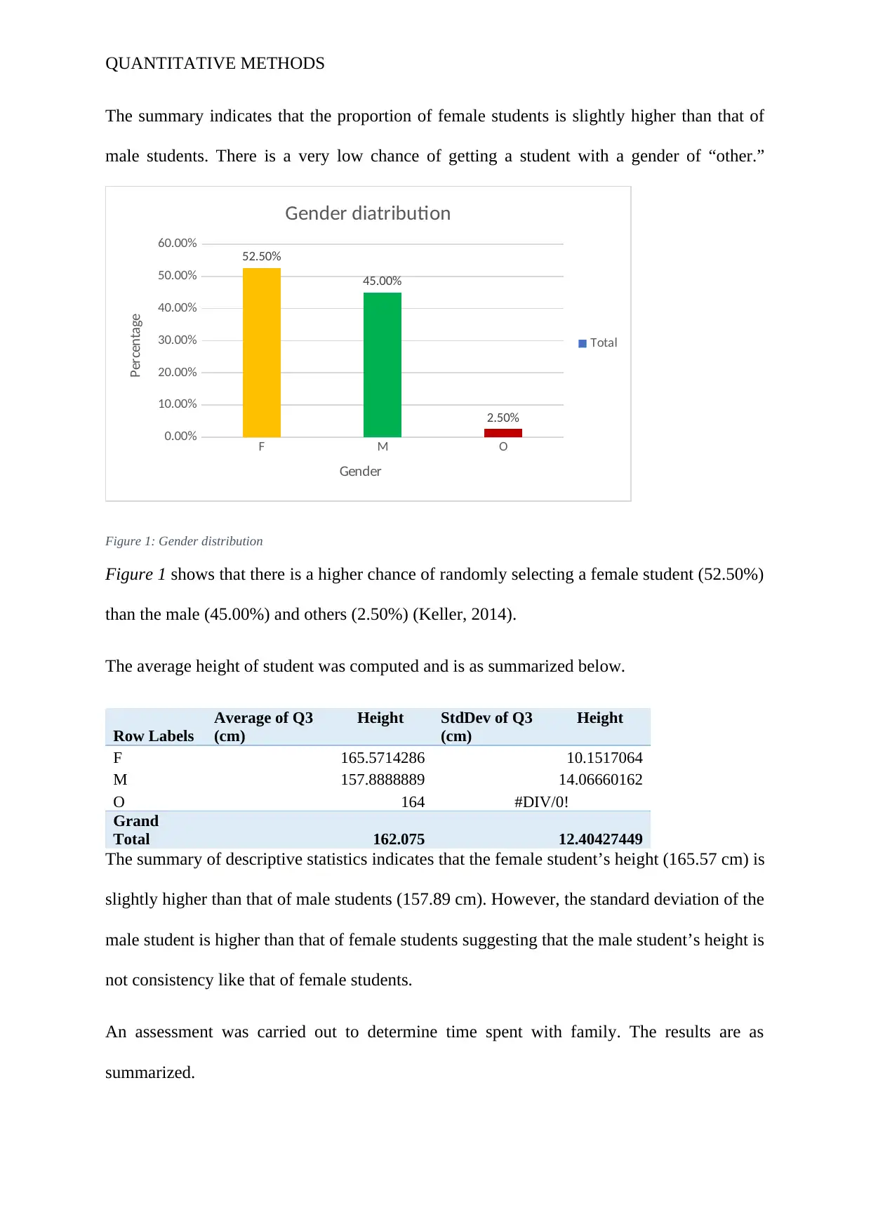
QUANTITATIVE METHODS
The summary indicates that the proportion of female students is slightly higher than that of
male students. There is a very low chance of getting a student with a gender of “other.”
F M O
0.00%
10.00%
20.00%
30.00%
40.00%
50.00%
60.00%
52.50%
45.00%
2.50%
Gender diatribution
Total
Gender
Percentage
Figure 1: Gender distribution
Figure 1 shows that there is a higher chance of randomly selecting a female student (52.50%)
than the male (45.00%) and others (2.50%) (Keller, 2014).
The average height of student was computed and is as summarized below.
Row Labels
Average of Q3 Height
(cm)
StdDev of Q3 Height
(cm)
F 165.5714286 10.1517064
M 157.8888889 14.06660162
O 164 #DIV/0!
Grand
Total 162.075 12.40427449
The summary of descriptive statistics indicates that the female student’s height (165.57 cm) is
slightly higher than that of male students (157.89 cm). However, the standard deviation of the
male student is higher than that of female students suggesting that the male student’s height is
not consistency like that of female students.
An assessment was carried out to determine time spent with family. The results are as
summarized.
⊘ This is a preview!⊘
Do you want full access?
Subscribe today to unlock all pages.
Trusted by 1+ million students worldwide
QUANTITATIVE METHODS
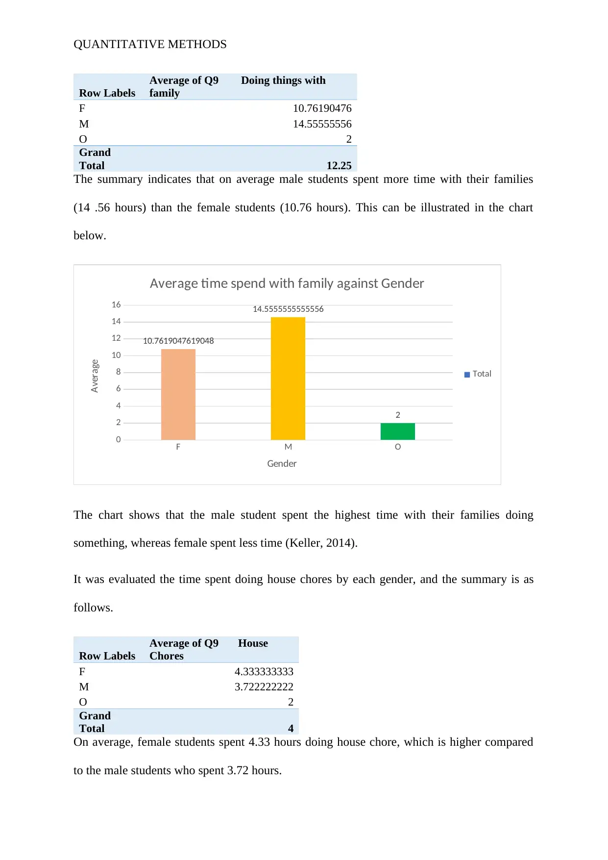
Row Labels
Average of Q9 Doing things with
family
F 10.76190476
M 14.55555556
O 2
Grand
Total 12.25
The summary indicates that on average male students spent more time with their families
(14 .56 hours) than the female students (10.76 hours). This can be illustrated in the chart
below.
F M O
0
2
4
6
8
10
12
14
16
10.7619047619048
14.5555555555556
2
Average time spend with family against Gender
Total
Gender
Average
The chart shows that the male student spent the highest time with their families doing
something, whereas female spent less time (Keller, 2014).
It was evaluated the time spent doing house chores by each gender, and the summary is as
follows.
Row Labels
Average of Q9 House
Chores
F 4.333333333
M 3.722222222
O 2
Grand
Total 4
On average, female students spent 4.33 hours doing house chore, which is higher compared
to the male students who spent 3.72 hours.
Row Labels
Average of Q9 Doing things with
family
F 10.76190476
M 14.55555556
O 2
Grand
Total 12.25
The summary indicates that on average male students spent more time with their families
(14 .56 hours) than the female students (10.76 hours). This can be illustrated in the chart
below.
F M O
0
2
4
6
8
10
12
14
16
10.7619047619048
14.5555555555556
2
Average time spend with family against Gender
Total
Gender
Average
The chart shows that the male student spent the highest time with their families doing
something, whereas female spent less time (Keller, 2014).
It was evaluated the time spent doing house chores by each gender, and the summary is as
follows.
Row Labels
Average of Q9 House
Chores
F 4.333333333
M 3.722222222
O 2
Grand
Total 4
On average, female students spent 4.33 hours doing house chore, which is higher compared
to the male students who spent 3.72 hours.
Paraphrase This Document
Need a fresh take? Get an instant paraphrase of this document with our AI Paraphraser
QUANTITATIVE METHODS
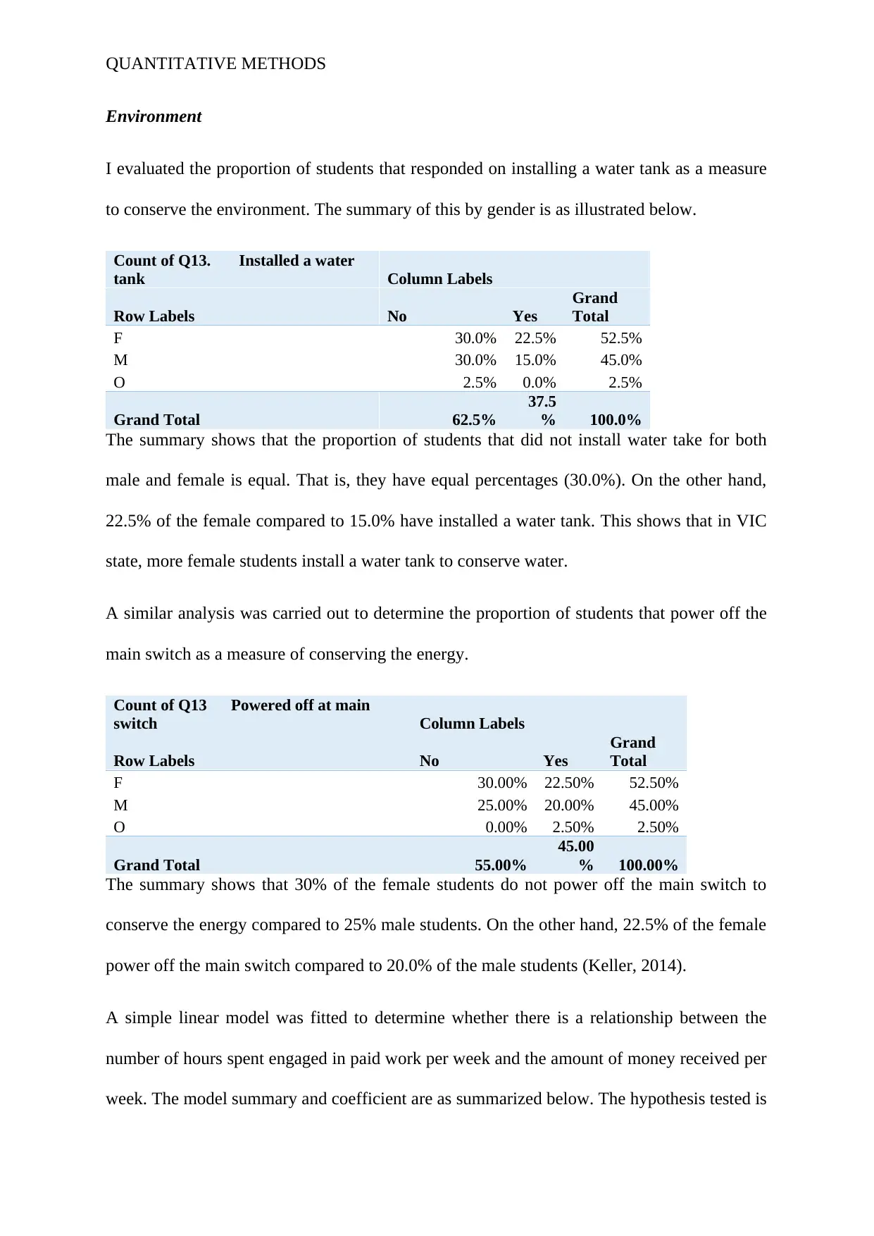
Environment
I evaluated the proportion of students that responded on installing a water tank as a measure
to conserve the environment. The summary of this by gender is as illustrated below.
Count of Q13. Installed a water
tank Column Labels
Row Labels No Yes
Grand
Total
F 30.0% 22.5% 52.5%
M 30.0% 15.0% 45.0%
O 2.5% 0.0% 2.5%
Grand Total 62.5%
37.5
% 100.0%
The summary shows that the proportion of students that did not install water take for both
male and female is equal. That is, they have equal percentages (30.0%). On the other hand,
22.5% of the female compared to 15.0% have installed a water tank. This shows that in VIC
state, more female students install a water tank to conserve water.
A similar analysis was carried out to determine the proportion of students that power off the
main switch as a measure of conserving the energy.
Count of Q13 Powered off at main
switch Column Labels
Row Labels No Yes
Grand
Total
F 30.00% 22.50% 52.50%
M 25.00% 20.00% 45.00%
O 0.00% 2.50% 2.50%
Grand Total 55.00%
45.00
% 100.00%
The summary shows that 30% of the female students do not power off the main switch to
conserve the energy compared to 25% male students. On the other hand, 22.5% of the female
power off the main switch compared to 20.0% of the male students (Keller, 2014).
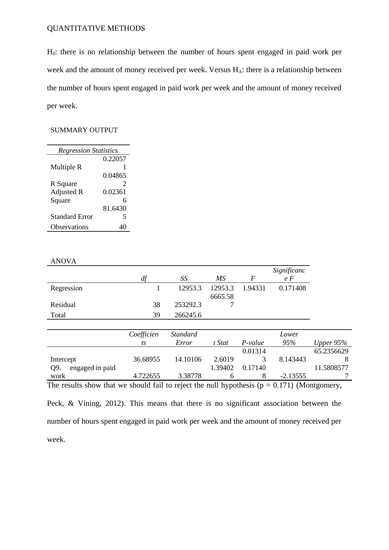
A simple linear model was fitted to determine whether there is a relationship between the
number of hours spent engaged in paid work per week and the amount of money received per
week. The model summary and coefficient are as summarized below. The hypothesis tested is
Environment
I evaluated the proportion of students that responded on installing a water tank as a measure
to conserve the environment. The summary of this by gender is as illustrated below.
Count of Q13. Installed a water
tank Column Labels
Row Labels No Yes
Grand
Total
F 30.0% 22.5% 52.5%
M 30.0% 15.0% 45.0%
O 2.5% 0.0% 2.5%
Grand Total 62.5%
37.5
% 100.0%
The summary shows that the proportion of students that did not install water take for both
male and female is equal. That is, they have equal percentages (30.0%). On the other hand,
22.5% of the female compared to 15.0% have installed a water tank. This shows that in VIC
state, more female students install a water tank to conserve water.
A similar analysis was carried out to determine the proportion of students that power off the
main switch as a measure of conserving the energy.
Count of Q13 Powered off at main
switch Column Labels
Row Labels No Yes
Grand
Total
F 30.00% 22.50% 52.50%
M 25.00% 20.00% 45.00%
O 0.00% 2.50% 2.50%
Grand Total 55.00%
45.00
% 100.00%
The summary shows that 30% of the female students do not power off the main switch to
conserve the energy compared to 25% male students. On the other hand, 22.5% of the female
power off the main switch compared to 20.0% of the male students (Keller, 2014).
A simple linear model was fitted to determine whether there is a relationship between the
number of hours spent engaged in paid work per week and the amount of money received per
week. The model summary and coefficient are as summarized below. The hypothesis tested is
QUANTITATIVE METHODS
H0: there is no relationship between the number of hours spent engaged in paid work per
week and the amount of money received per week. Versus HA: there is a relationship between
the number of hours spent engaged in paid work per week and the amount of money received
per week.
SUMMARY OUTPUT
Regression Statistics
Multiple R
0.22057
1
R Square
0.04865
2
Adjusted R
Square
0.02361
6
Standard Error
81.6430
5
Observations 40
ANOVA
df SS MS F
Significanc
e F
Regression 1 12953.3 12953.3 1.94331 0.171408
Residual 38 253292.3
6665.58
7
Total 39 266245.6
Coefficien
ts
Standard
Error t Stat P-value
Lower
95% Upper 95%
Intercept 36.68955 14.10106 2.6019
0.01314
3 8.143443
65.2356629
8
Q9. engaged in paid
work 4.722655 3.38778
1.39402
6
0.17140
8 -2.13555
11.5808577
7
The results show that we should fail to reject the null hypothesis (p = 0.171) (Montgomery,
Peck, & Vining, 2012). This means that there is no significant association between the
number of hours spent engaged in paid work per week and the amount of money received per
week.
⊘ This is a preview!⊘
Do you want full access?
Subscribe today to unlock all pages.
Trusted by 1+ million students worldwide
QUANTITATIVE METHODS
NSW data analysis
An assess met was carried out to determine the distribution of gender in the NSW sample
data.
Table 2: Gender distribution
Row Labels
Count of Q2
Gender
F 57.50%
M 42.50%
Grand
Total 100.00%
The summary shows that the proportion of males is lower than that of the female students in
VIC state. That is, there is a 42.50 % chance of randomly selecting a male student whereas
there is a 57.50 % chance of randomly selecting a female student (Keller, 2014). This
distribution is as illustrated below.
F M
0.00%
10.00%
20.00%
30.00%
40.00%
50.00%
60.00%
70.00%
57.50%
42.50%
Gender distribution
Total
Gender
Percentage
Figure 2: Gender distribution
The chart indicates that there is a higher number of female students than the male students.
Second, an assessment of descriptive statistics of the height of students by gender.
Row Labels
Average of Q3 Height
(cm)
StdDev of Q3 Height
(cm)
F 155.4347826 12.54383618
M 159.8823529 13.94579844
Grand 157.325 13.17220753
Paraphrase This Document
Need a fresh take? Get an instant paraphrase of this document with our AI Paraphraser
QUANTITATIVE METHODS
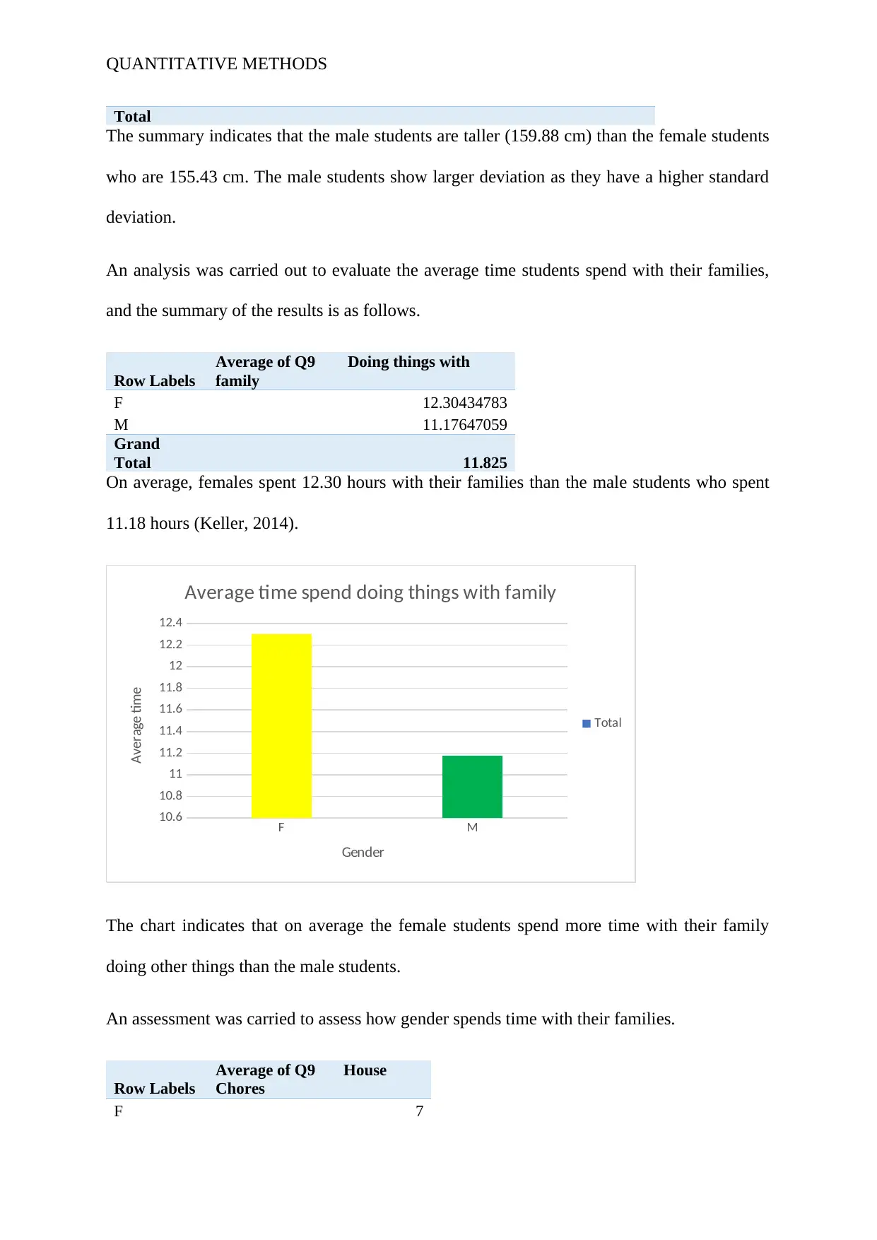
Total
The summary indicates that the male students are taller (159.88 cm) than the female students
who are 155.43 cm. The male students show larger deviation as they have a higher standard
deviation.
An analysis was carried out to evaluate the average time students spend with their families,
and the summary of the results is as follows.
Row Labels
Average of Q9 Doing things with
family
F 12.30434783
M 11.17647059
Grand
Total 11.825
On average, females spent 12.30 hours with their families than the male students who spent
11.18 hours (Keller, 2014).
F M
10.6
10.8
11
11.2
11.4
11.6
11.8
12
12.2
12.4
Average time spend doing things with family
Total
Gender
Average time
The chart indicates that on average the female students spend more time with their family
doing other things than the male students.
An assessment was carried to assess how gender spends time with their families.
Row Labels
Average of Q9 House
Chores
F 7
Total
The summary indicates that the male students are taller (159.88 cm) than the female students
who are 155.43 cm. The male students show larger deviation as they have a higher standard
deviation.
An analysis was carried out to evaluate the average time students spend with their families,
and the summary of the results is as follows.
Row Labels
Average of Q9 Doing things with
family
F 12.30434783
M 11.17647059
Grand
Total 11.825
On average, females spent 12.30 hours with their families than the male students who spent
11.18 hours (Keller, 2014).
F M
10.6
10.8
11
11.2
11.4
11.6
11.8
12
12.2
12.4
Average time spend doing things with family
Total
Gender
Average time
The chart indicates that on average the female students spend more time with their family
doing other things than the male students.
An assessment was carried to assess how gender spends time with their families.
Row Labels
Average of Q9 House
Chores
F 7
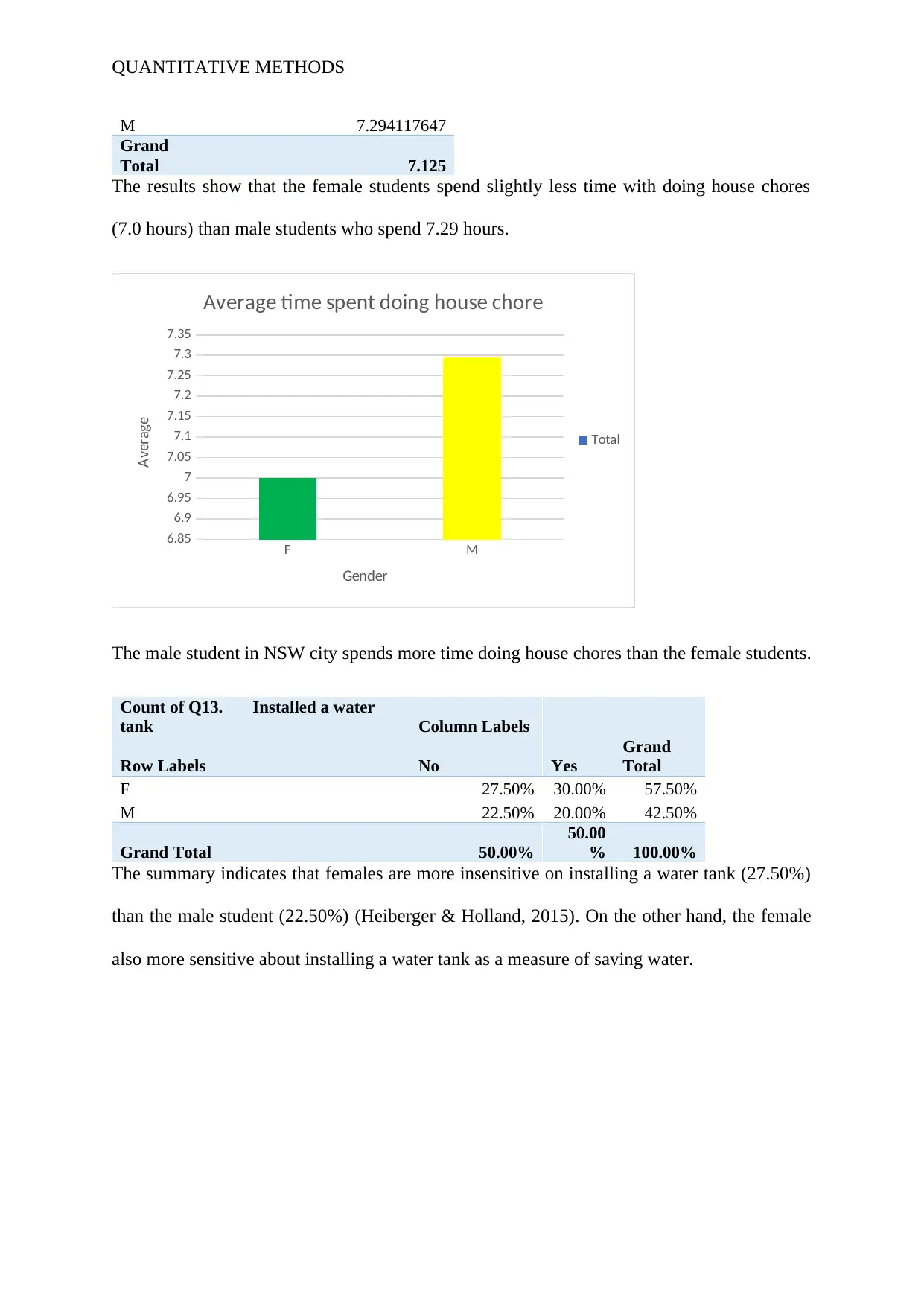
QUANTITATIVE METHODS
M 7.294117647
Grand
Total 7.125
The results show that the female students spend slightly less time with doing house chores
(7.0 hours) than male students who spend 7.29 hours.
F M
6.85
6.9
6.95
7
7.05
7.1
7.15
7.2
7.25
7.3
7.35
Average time spent doing house chore
Total
Gender
Average
The male student in NSW city spends more time doing house chores than the female students.
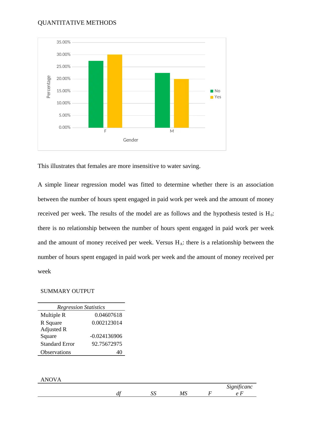
Count of Q13. Installed a water
tank Column Labels
Row Labels No Yes
Grand
Total
F 27.50% 30.00% 57.50%
M 22.50% 20.00% 42.50%
Grand Total 50.00%
50.00
% 100.00%
The summary indicates that females are more insensitive on installing a water tank (27.50%)
than the male student (22.50%) (Heiberger & Holland, 2015). On the other hand, the female
also more sensitive about installing a water tank as a measure of saving water.
M 7.294117647
Grand
Total 7.125
The results show that the female students spend slightly less time with doing house chores
(7.0 hours) than male students who spend 7.29 hours.
F M
6.85
6.9
6.95
7
7.05
7.1
7.15
7.2
7.25
7.3
7.35
Average time spent doing house chore
Total
Gender
Average
The male student in NSW city spends more time doing house chores than the female students.
Count of Q13. Installed a water
tank Column Labels
Row Labels No Yes
Grand
Total
F 27.50% 30.00% 57.50%
M 22.50% 20.00% 42.50%
Grand Total 50.00%
50.00
% 100.00%
The summary indicates that females are more insensitive on installing a water tank (27.50%)
than the male student (22.50%) (Heiberger & Holland, 2015). On the other hand, the female
also more sensitive about installing a water tank as a measure of saving water.
⊘ This is a preview!⊘
Do you want full access?
Subscribe today to unlock all pages.
Trusted by 1+ million students worldwide
QUANTITATIVE METHODS
F M
0.00%
5.00%
10.00%
15.00%
20.00%
25.00%
30.00%
35.00%
No
Yes
Gender
Percentage
This illustrates that females are more insensitive to water saving.
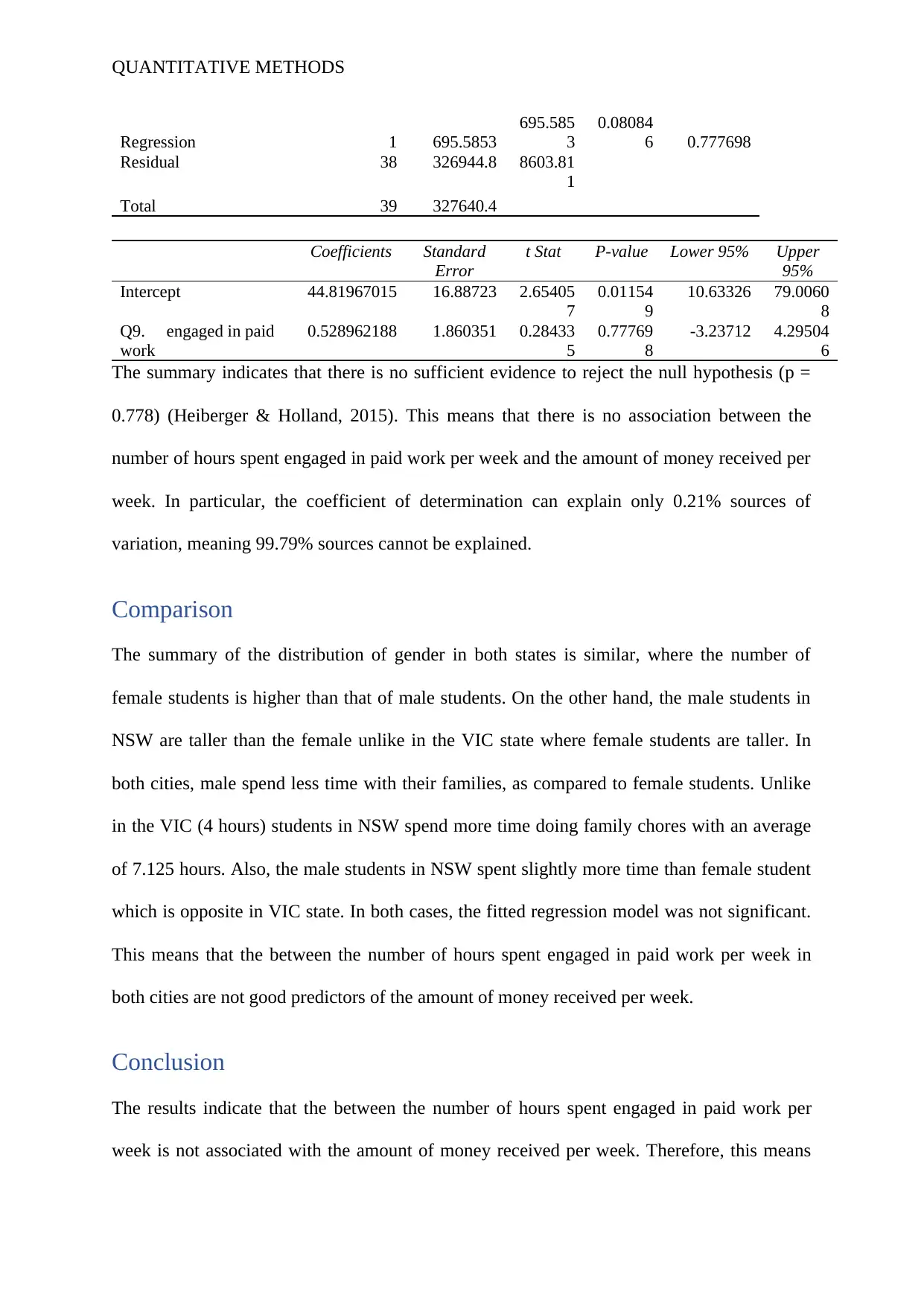
A simple linear regression model was fitted to determine whether there is an association
between the number of hours spent engaged in paid work per week and the amount of money
received per week. The results of the model are as follows and the hypothesis tested is H0:
there is no relationship between the number of hours spent engaged in paid work per week
and the amount of money received per week. Versus HA: there is a relationship between the
number of hours spent engaged in paid work per week and the amount of money received per
week
SUMMARY OUTPUT
Regression Statistics
Multiple R 0.04607618
R Square 0.002123014
Adjusted R
Square -0.024136906
Standard Error 92.75672975
Observations 40
ANOVA
df SS MS F
Significanc
e F
F M
0.00%
5.00%
10.00%
15.00%
20.00%
25.00%
30.00%
35.00%
No
Yes
Gender
Percentage
This illustrates that females are more insensitive to water saving.
A simple linear regression model was fitted to determine whether there is an association
between the number of hours spent engaged in paid work per week and the amount of money
received per week. The results of the model are as follows and the hypothesis tested is H0:
there is no relationship between the number of hours spent engaged in paid work per week
and the amount of money received per week. Versus HA: there is a relationship between the
number of hours spent engaged in paid work per week and the amount of money received per
week
SUMMARY OUTPUT
Regression Statistics
Multiple R 0.04607618
R Square 0.002123014
Adjusted R
Square -0.024136906
Standard Error 92.75672975
Observations 40
ANOVA
df SS MS F
Significanc
e F
Paraphrase This Document
Need a fresh take? Get an instant paraphrase of this document with our AI Paraphraser
QUANTITATIVE METHODS
Regression 1 695.5853
695.585
3
0.08084
6 0.777698
Residual 38 326944.8 8603.81
1
Total 39 327640.4
Coefficients Standard
Error
t Stat P-value Lower 95% Upper
95%
Intercept 44.81967015 16.88723 2.65405
7
0.01154
9
10.63326 79.0060
8
Q9. engaged in paid
work
0.528962188 1.860351 0.28433
5
0.77769
8
-3.23712 4.29504
6
The summary indicates that there is no sufficient evidence to reject the null hypothesis (p =
0.778) (Heiberger & Holland, 2015). This means that there is no association between the
number of hours spent engaged in paid work per week and the amount of money received per
week. In particular, the coefficient of determination can explain only 0.21% sources of
variation, meaning 99.79% sources cannot be explained.
Comparison
The summary of the distribution of gender in both states is similar, where the number of
female students is higher than that of male students. On the other hand, the male students in
NSW are taller than the female unlike in the VIC state where female students are taller. In
both cities, male spend less time with their families, as compared to female students. Unlike
in the VIC (4 hours) students in NSW spend more time doing family chores with an average
of 7.125 hours. Also, the male students in NSW spent slightly more time than female student
which is opposite in VIC state. In both cases, the fitted regression model was not significant.
This means that the between the number of hours spent engaged in paid work per week in
both cities are not good predictors of the amount of money received per week.
Conclusion
The results indicate that the between the number of hours spent engaged in paid work per
week is not associated with the amount of money received per week. Therefore, this means
QUANTITATIVE METHODS
that the number of hours engaged in paid work cannot be used as a determinant of income or
money received by students. The research indicated that female students in both cities are
more sensitive than the male students in Installing a water tank as a measure of conserving
water. Therefore, there is a need to enlighten the male students on the need to conserve the
water.
References
Barton, M., Yeatts, P. E., Henson, R. K., & Martin, S. B. (2016). Moving beyond univariate
post-hoc testing in exercise science: A primer on descriptive discriminate analysis.
Research quarterly for exercise and sport, 87(4), 365-375.
Heiberger, R. M., & Holland, B. (2015). Multiple Regression—Regression Diagnostics.
Statistical Analysis and Data Display, 345-375.
Keller, G. (2014). Statistics for management and economics. Nelson Education.
Montgomery, D. C., Peck, E. A., & Vining, G. G. (2012). Introduction to linear regression
analysis. 821. John Wiley & Sons.
⊘ This is a preview!⊘
Do you want full access?
Subscribe today to unlock all pages.
Trusted by 1+ million students worldwide
1 out of 13

Your All-in-One AI-Powered Toolkit for Academic Success.
+13062052269
info@desklib.com
Available 24*7 on WhatsApp / Email
![[object Object]](/_next/static/media/star-bottom.7253800d.svg)
Unlock your academic potential
Copyright © 2020–2026 A2Z Services. All Rights Reserved. Developed and managed by ZUCOL.