Statistical Modelling Assignment: Analysis of Gender Wage Differences

This statistical modelling assignment investigates the gender wage gap in Australia using both secondary data from the Australian Taxation Office (ATO) and primary data collected through a survey. The analysis begins with descriptive statistics, exploring relationships between gender, occupation, salary, and deductions. Multiple bar graphs and scatterplots visually represent these relationships, highlighting the disparity in wages between men and women across different occupations. Numerical summaries of income, including mean, median, standard deviation, and skewness, further quantify these differences. The study then moves to inferential statistics, utilizing z-tests and t-tests to assess the significance of observed wage differences. Hypothesis testing is employed to determine if the proportion of male employees in certain occupations exceeds a threshold and if there are significant differences in the average income between genders. The findings consistently reveal a substantial gender wage gap, regardless of the occupation or data source, although the variable of age has not been considered in the analysis. The assignment concludes by summarizing the key findings and acknowledging limitations, such as the exclusion of age-related factors, and suggesting avenues for future research.

Running Head: STATISTICAL MODELLING ASSIGNMENT
Statistical Modelling Assignment
Name of the Student
Name of the University
Author Note

1STATISTICAL MODELLING ASSIGNMENT
Table of Contents
Section 1: Introduction................................................................................................................................2
Section 2: Descriptive Statistics...................................................................................................................2
Section 3: Inferential Statistics....................................................................................................................4
Section 4: Discussion and Conclusion..........................................................................................................6
References...................................................................................................................................................8

2STATISTICAL MODELLING ASSIGNMENT
Section 1: Introduction
In Australia, there are differences in the salaries of men and women. This difference in salary is
known as gender gap or gender inequality. There are various reasons for this gender discrimination. One
of the major reasons id that there are discriminations at the time of hiring. Other than that, the salary
structure of the industries in which women are working might be different from the salary structure in
which women are working (Australia 2014). A lot of other reasons are also existent. This study is aimed
mostly towards assessing the different aspects affecting the occupation and salary for different gender.
The most important thing that is necessary for conducting this research is data which has been
collected from the website of Australian Taxation Office (ATO). The dataset considered is a subset of the
original dataset available in ATO website. Data on 1000 Australian people have been sampled to form
the subset for the study. Information about variables such as gender, occupation of the respondents,
the salary of the respondents, deductions from salary for gifts and donations are stored in the dataset
retrieved from the ATO website. As the data is collected from the ATO website, and not collected
directly from the field of survey for the purpose of the analysis, this data is known as secondary data.
The variables gender and occupation are categorical variables and the variables salary and deductions
are numeric variables.
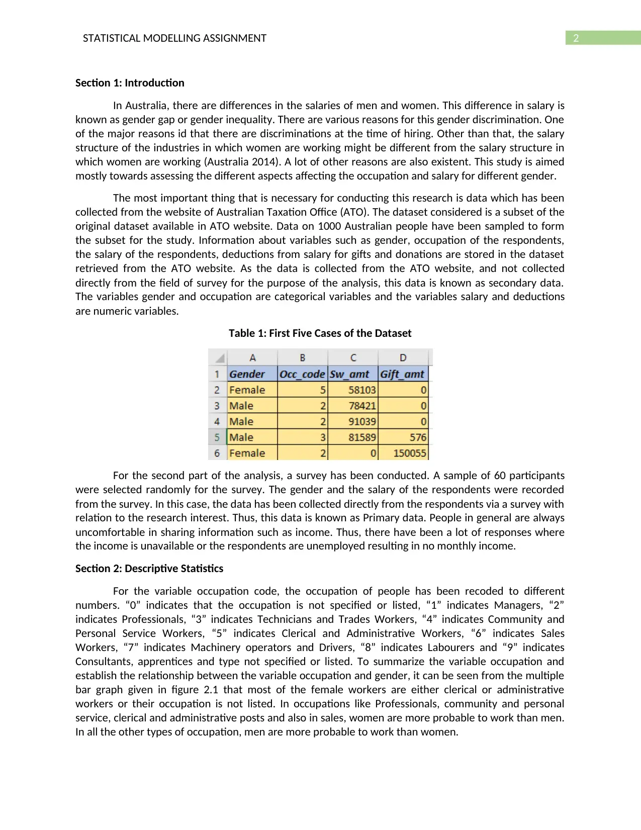
Table 1: First Five Cases of the Dataset
For the second part of the analysis, a survey has been conducted. A sample of 60 participants
were selected randomly for the survey. The gender and the salary of the respondents were recorded
from the survey. In this case, the data has been collected directly from the respondents via a survey with
relation to the research interest. Thus, this data is known as Primary data. People in general are always
uncomfortable in sharing information such as income. Thus, there have been a lot of responses where
the income is unavailable or the respondents are unemployed resulting in no monthly income.
Section 2: Descriptive Statistics
For the variable occupation code, the occupation of people has been recoded to different
numbers. “0” indicates that the occupation is not specified or listed, “1” indicates Managers, “2”
indicates Professionals, “3” indicates Technicians and Trades Workers, “4” indicates Community and
Personal Service Workers, “5” indicates Clerical and Administrative Workers, “6” indicates Sales
Workers, “7” indicates Machinery operators and Drivers, “8” indicates Labourers and “9” indicates
Consultants, apprentices and type not specified or listed. To summarize the variable occupation and
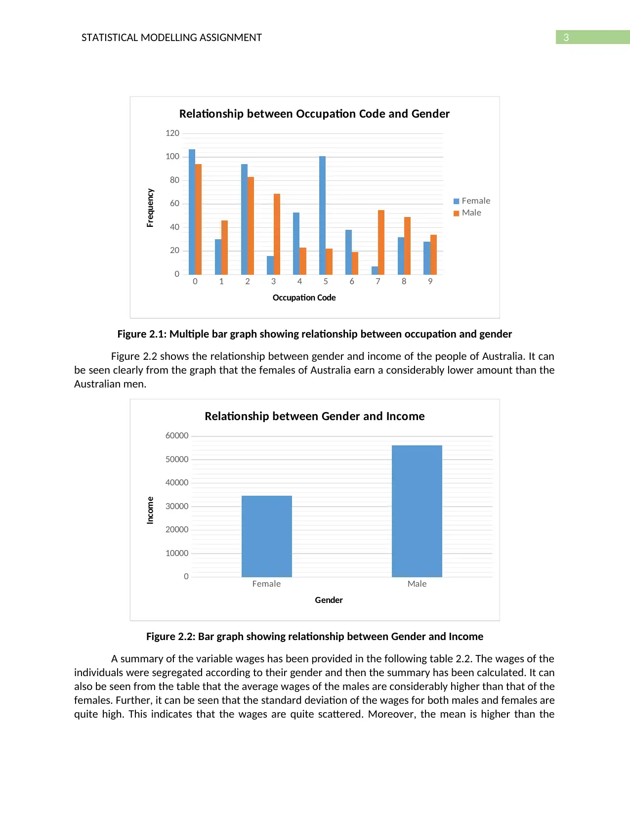
establish the relationship between the variable occupation and gender, it can be seen from the multiple
bar graph given in figure 2.1 that most of the female workers are either clerical or administrative
workers or their occupation is not listed. In occupations like Professionals, community and personal
service, clerical and administrative posts and also in sales, women are more probable to work than men.
In all the other types of occupation, men are more probable to work than women.

3STATISTICAL MODELLING ASSIGNMENT
0 1 2 3 4 5 6 7 8 9
0
20
40
60
80
100
120
Relationship between Occupation Code and Gender
Female
Male
Occupation Code
Frequency
Figure 2.1: Multiple bar graph showing relationship between occupation and gender
Figure 2.2 shows the relationship between gender and income of the people of Australia. It can
be seen clearly from the graph that the females of Australia earn a considerably lower amount than the
Australian men.
Female Male
0
10000
20000
30000
40000
50000
60000
Relationship between Gender and Income
Gender
Income
Figure 2.2: Bar graph showing relationship between Gender and Income
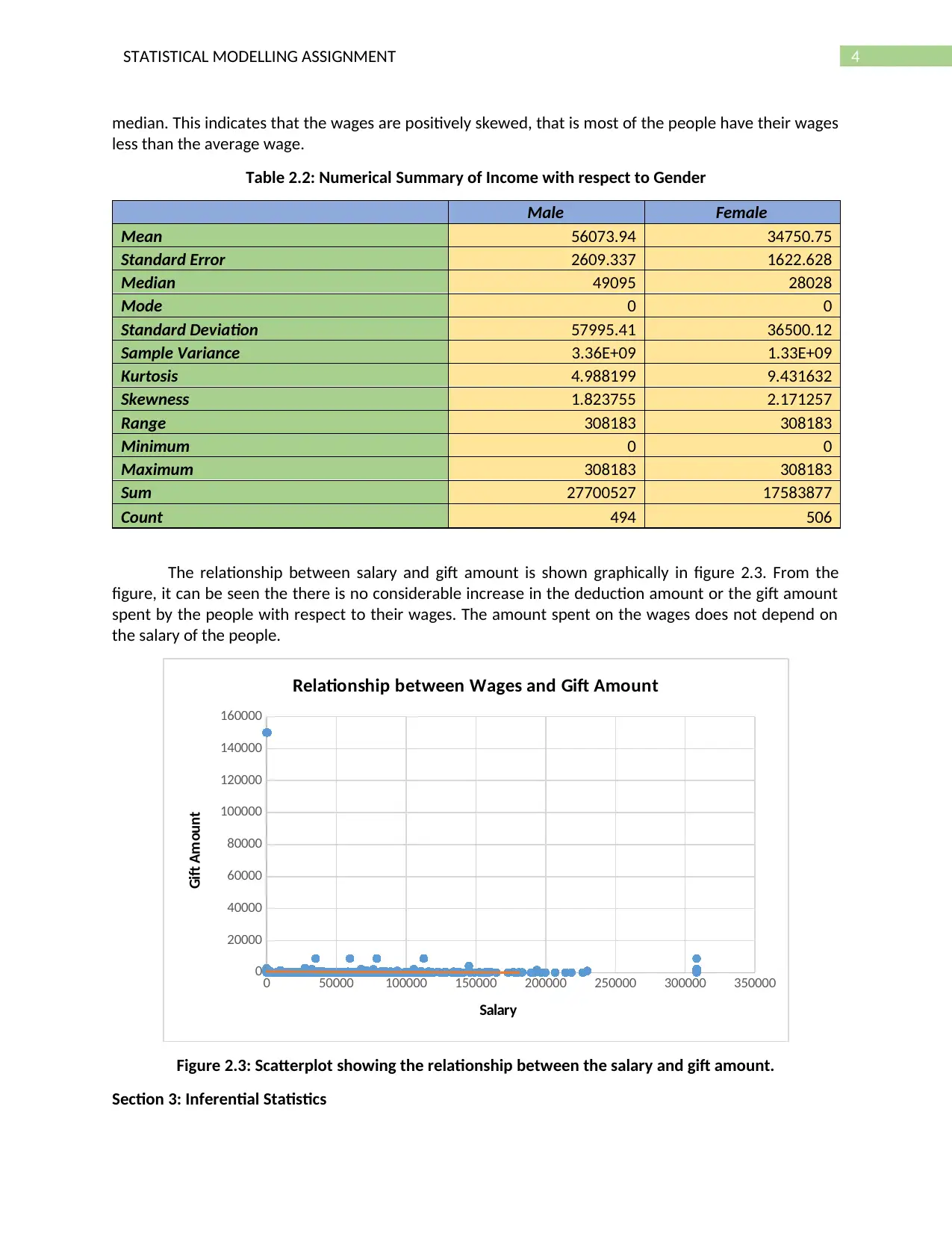
A summary of the variable wages has been provided in the following table 2.2. The wages of the
individuals were segregated according to their gender and then the summary has been calculated. It can
also be seen from the table that the average wages of the males are considerably higher than that of the
females. Further, it can be seen that the standard deviation of the wages for both males and females are
quite high. This indicates that the wages are quite scattered. Moreover, the mean is higher than the

4STATISTICAL MODELLING ASSIGNMENT
median. This indicates that the wages are positively skewed, that is most of the people have their wages
less than the average wage.
Table 2.2: Numerical Summary of Income with respect to Gender
Male Female
Mean 56073.94 34750.75
Standard Error 2609.337 1622.628
Median 49095 28028
Mode 0 0
Standard Deviation 57995.41 36500.12
Sample Variance 3.36E+09 1.33E+09
Kurtosis 4.988199 9.431632
Skewness 1.823755 2.171257
Range 308183 308183
Minimum 0 0
Maximum 308183 308183
Sum 27700527 17583877
Count 494 506
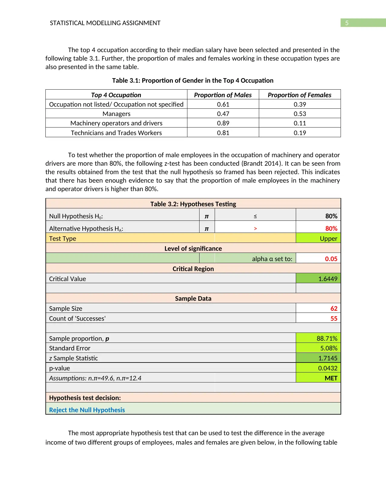
The relationship between salary and gift amount is shown graphically in figure 2.3. From the
figure, it can be seen the there is no considerable increase in the deduction amount or the gift amount
spent by the people with respect to their wages. The amount spent on the wages does not depend on
the salary of the people.
0 50000 100000 150000 200000 250000 300000 350000
0
20000
40000
60000
80000
100000
120000
140000
160000
Relationship between Wages and Gift Amount
Salary
Gift Amount
Figure 2.3: Scatterplot showing the relationship between the salary and gift amount.
Section 3: Inferential Statistics

5STATISTICAL MODELLING ASSIGNMENT
The top 4 occupation according to their median salary have been selected and presented in the
following table 3.1. Further, the proportion of males and females working in these occupation types are
also presented in the same table.
Table 3.1: Proportion of Gender in the Top 4 Occupation
Top 4 Occupation Proportion of Males Proportion of Females
Occupation not listed/ Occupation not specified 0.61 0.39
Managers 0.47 0.53
Machinery operators and drivers 0.89 0.11
Technicians and Trades Workers 0.81 0.19
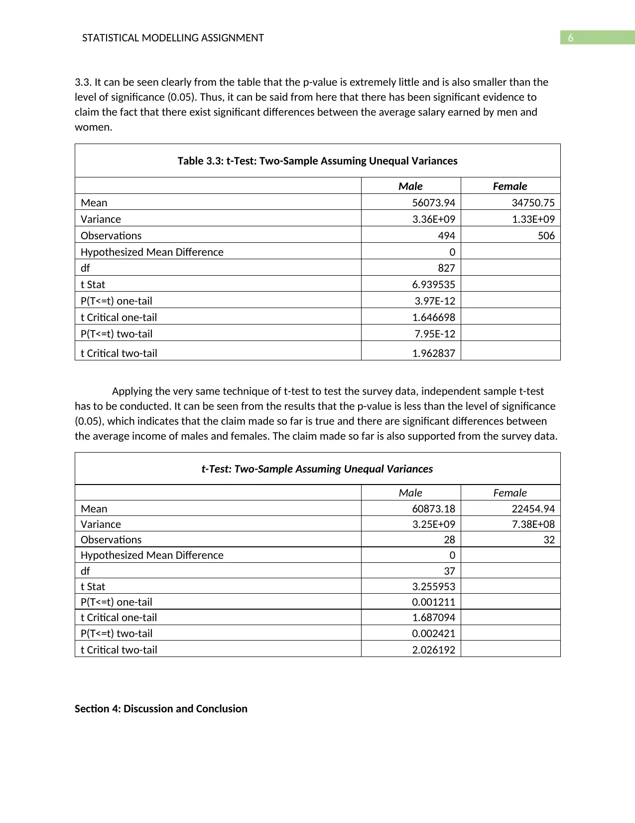
To test whether the proportion of male employees in the occupation of machinery and operator
drivers are more than 80%, the following z-test has been conducted (Brandt 2014). It can be seen from
the results obtained from the test that the null hypothesis so framed has been rejected. This indicates
that there has been enough evidence to say that the proportion of male employees in the machinery
and operator drivers is higher than 80%.
Table 3.2: Hypotheses Testing
Null Hypothesis H0: π ≤ 80%
Alternative Hypothesis HA: π > 80%
Test Type Upper
Level of significance
alpha α set to: 0.05
Critical Region
Critical Value 1.6449
Sample Data
Sample Size 62
Count of 'Successes' 55
Sample proportion, p 88.71%
Standard Error 5.08%
z Sample Statistic 1.7145
p-value 0.0432
Assumptions: n.π=49.6, n.π=12.4 MET
Hypothesis test decision:
Reject the Null Hypothesis
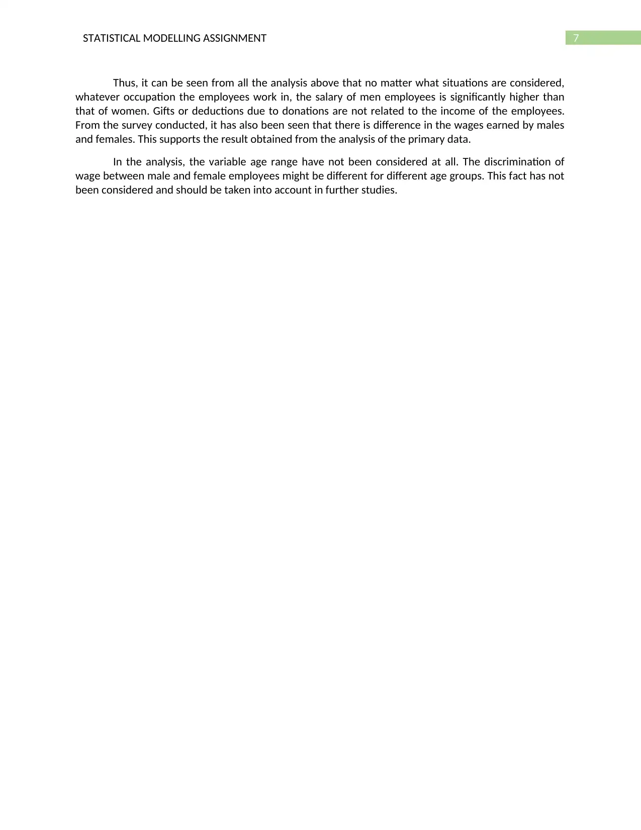
The most appropriate hypothesis test that can be used to test the difference in the average
income of two different groups of employees, males and females are given below, in the following table

6STATISTICAL MODELLING ASSIGNMENT
3.3. It can be seen clearly from the table that the p-value is extremely little and is also smaller than the
level of significance (0.05). Thus, it can be said from here that there has been significant evidence to
claim the fact that there exist significant differences between the average salary earned by men and
women.
Table 3.3: t-Test: Two-Sample Assuming Unequal Variances
Male Female
Mean 56073.94 34750.75
Variance 3.36E+09 1.33E+09
Observations 494 506
Hypothesized Mean Difference 0
df 827
t Stat 6.939535
P(T<=t) one-tail 3.97E-12
t Critical one-tail 1.646698
P(T<=t) two-tail 7.95E-12
t Critical two-tail 1.962837
Applying the very same technique of t-test to test the survey data, independent sample t-test
has to be conducted. It can be seen from the results that the p-value is less than the level of significance
(0.05), which indicates that the claim made so far is true and there are significant differences between
the average income of males and females. The claim made so far is also supported from the survey data.
t-Test: Two-Sample Assuming Unequal Variances
Male Female
Mean 60873.18 22454.94
Variance 3.25E+09 7.38E+08
Observations 28 32
Hypothesized Mean Difference 0
df 37
t Stat 3.255953
P(T<=t) one-tail 0.001211
t Critical one-tail 1.687094
P(T<=t) two-tail 0.002421
t Critical two-tail 2.026192
Section 4: Discussion and Conclusion

7STATISTICAL MODELLING ASSIGNMENT
Thus, it can be seen from all the analysis above that no matter what situations are considered,
whatever occupation the employees work in, the salary of men employees is significantly higher than
that of women. Gifts or deductions due to donations are not related to the income of the employees.
From the survey conducted, it has also been seen that there is difference in the wages earned by males
and females. This supports the result obtained from the analysis of the primary data.
In the analysis, the variable age range have not been considered at all. The discrimination of
wage between male and female employees might be different for different age groups. This fact has not
been considered and should be taken into account in further studies.

8STATISTICAL MODELLING ASSIGNMENT
References
Australia, G.C., 2014. An analysis of the gender wage gap in the Australian graduate labour market,
2013. Melbourne, Australia: Graduate Careers Australia.
Brandt, S., 2014. Testing Statistical Hypotheses. In Data Analysis (pp. 175-207). Springer, Cham.