Economics Assignment: Analyzing Auto Sales, Regression Model Problems

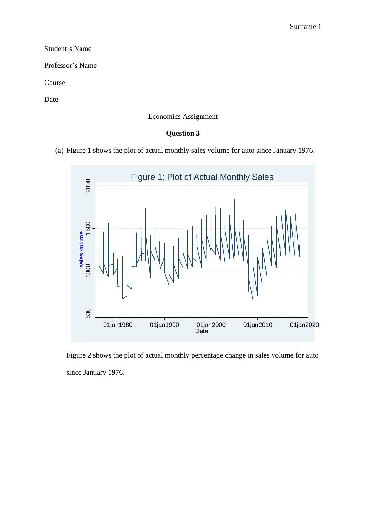
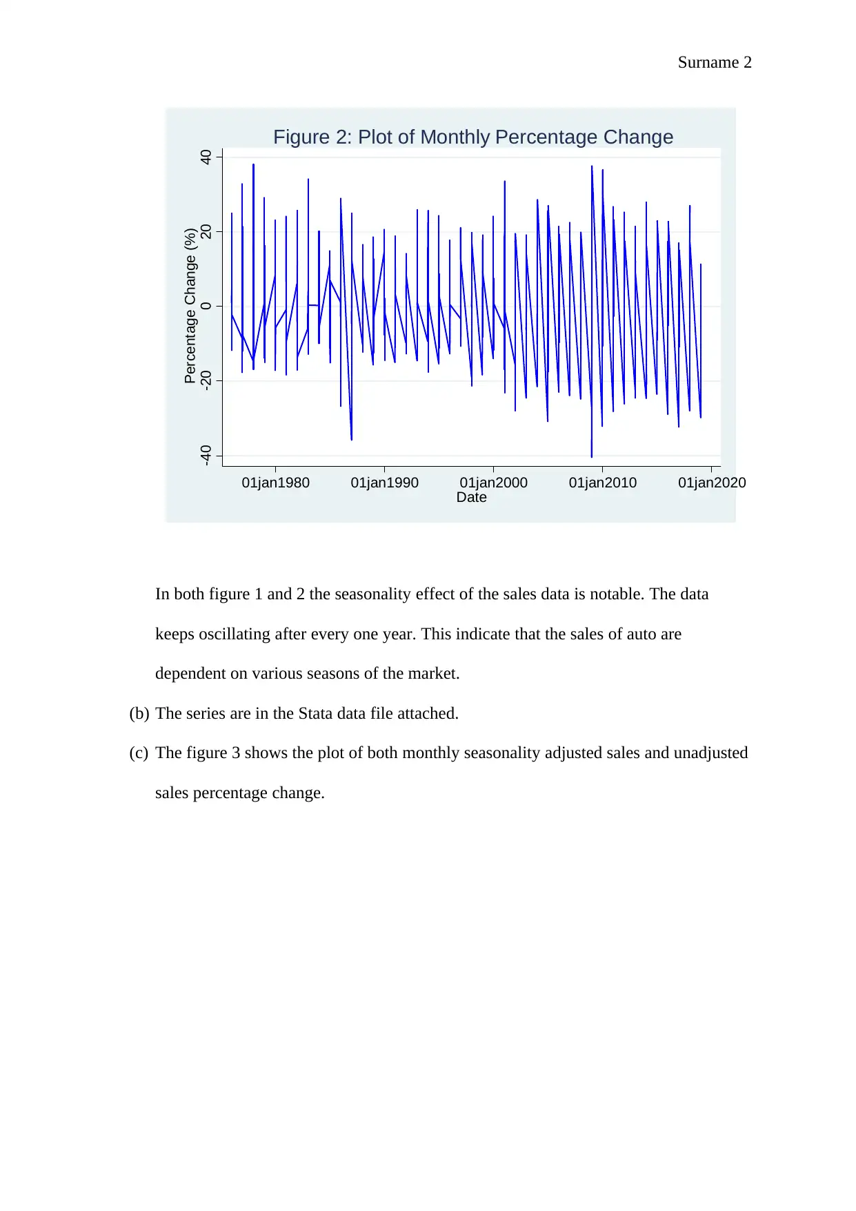
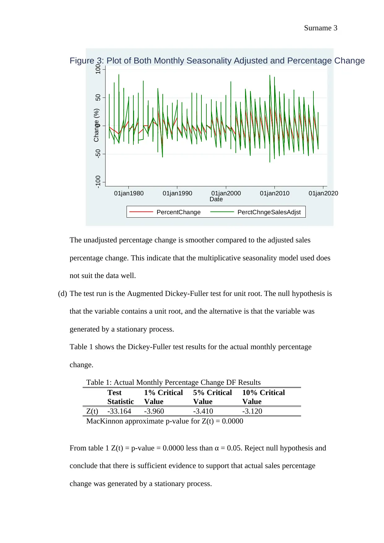
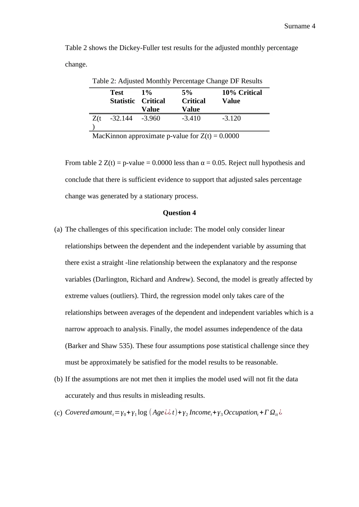
This economics assignment delves into the analysis of auto sales data from January 1976, examining both actual monthly sales volume and percentage changes, highlighting the seasonality effect evident in the data. It further explores the impact of seasonality adjustment on sales data and conducts Augmented Dickey-Fuller tests to assess data stationarity. The assignment also addresses the challenges associated with linear regression models, including assumptions about linearity, sensitivity to outliers, and independence of data, discussing the implications of violating these assumptions and proposing a regression model for covered amounts. Desklib provides access to similar solved assignments and past papers for students.

Surname 1
Student’s Name
Professor’s Name
Course
Date
Economics Assignment
Question 3
(a) Figure 1 shows the plot of actual monthly sales volume for auto since January 1976.
500 1000 1500 2000
sales volume
01jan1980 01jan1990 01jan2000 01jan2010 01jan2020
Date
Figure 1: Plot of Actual Monthly Sales
Figure 2 shows the plot of actual monthly percentage change in sales volume for auto
since January 1976.

Surname 2
-40 -20 0 20 40
Percentage Change (%)
01jan1980 01jan1990 01jan2000 01jan2010 01jan2020
Date
Figure 2: Plot of Monthly Percentage Change
In both figure 1 and 2 the seasonality effect of the sales data is notable. The data
keeps oscillating after every one year. This indicate that the sales of auto are
dependent on various seasons of the market.
(b) The series are in the Stata data file attached.
(c) The figure 3 shows the plot of both monthly seasonality adjusted sales and unadjusted
sales percentage change.

Surname 3
-100 -50 0 50 100Change (%)
01jan1980 01jan1990 01jan2000 01jan2010 01jan2020
Date
PercentChange PerctChngeSalesAdjst
Figure 3: Plot of Both Monthly Seasonality Adjusted and Percentage Change
The unadjusted percentage change is smoother compared to the adjusted sales
percentage change. This indicate that the multiplicative seasonality model used does
not suit the data well.
(d) The test run is the Augmented Dickey-Fuller test for unit root. The null hypothesis is
that the variable contains a unit root, and the alternative is that the variable was
generated by a stationary process.
Table 1 shows the Dickey-Fuller test results for the actual monthly percentage
change.
Table 1: Actual Monthly Percentage Change DF Results
Test
Statistic
1% Critical
Value
5% Critical
Value
10% Critical
Value
Z(t) -33.164 -3.960 -3.410 -3.120
MacKinnon approximate p-value for Z(t) = 0.0000
From table 1 Z(t) = p-value = 0.0000 less than α = 0.05. Reject null hypothesis and
conclude that there is sufficient evidence to support that actual sales percentage
change was generated by a stationary process.

Surname 4
Table 2 shows the Dickey-Fuller test results for the adjusted monthly percentage
change.
Table 2: Adjusted Monthly Percentage Change DF Results
Test
Statistic
1%
Critical
Value
5%
Critical
Value
10% Critical
Value
Z(t
)
-32.144 -3.960 -3.410 -3.120
MacKinnon approximate p-value for Z(t) = 0.0000
From table 2 Z(t) = p-value = 0.0000 less than α = 0.05. Reject null hypothesis and
conclude that there is sufficient evidence to support that adjusted sales percentage
change was generated by a stationary process.
Question 4
(a) The challenges of this specification include: The model only consider linear
relationships between the dependent and the independent variable by assuming that
there exist a straight -line relationship between the explanatory and the response
variables (Darlington, Richard and Andrew). Second, the model is greatly affected by
extreme values (outliers). Third, the regression model only takes care of the
relationships between averages of the dependent and independent variables which is a
narrow approach to analysis. Finally, the model assumes independence of the data
(Barker and Shaw 535). These four assumptions pose statistical challenge since they
must be approximately be satisfied for the model results to be reasonable.
(b) If the assumptions are not met then it implies the model used will not fit the data
accurately and thus results in misleading results.
(c) Covered amountt =γ0 + γ1 log ( Age¿¿ t)+ γ2 Incomet + γ3 Occupationt + Γ Ωit ¿

Surname 5
Work Cited
Barker, Lawrence E., and Kate M. Shaw. "Best (but oft-forgotten) practices: checking
assumptions concerning regression residuals." The American journal of clinical
nutrition102.3 (2015): 533-539.
Darlington, Richard B., and Andrew F. Hayes. Regression analysis and linear models:
Concepts, applications, and implementation. Guilford Publications, 2016.