Regression Analysis: Exploring Vehicle Ownership Factors in Europe

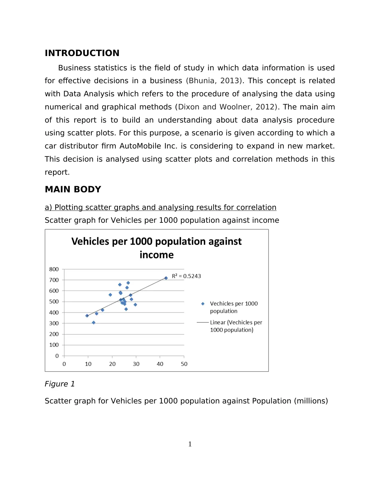
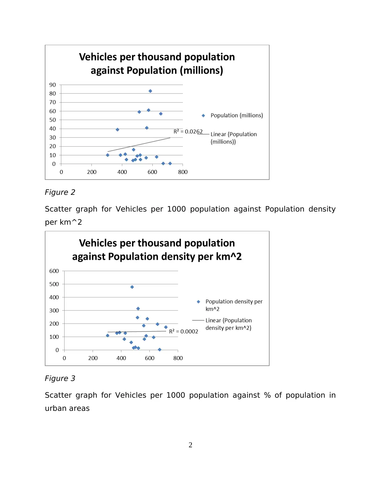
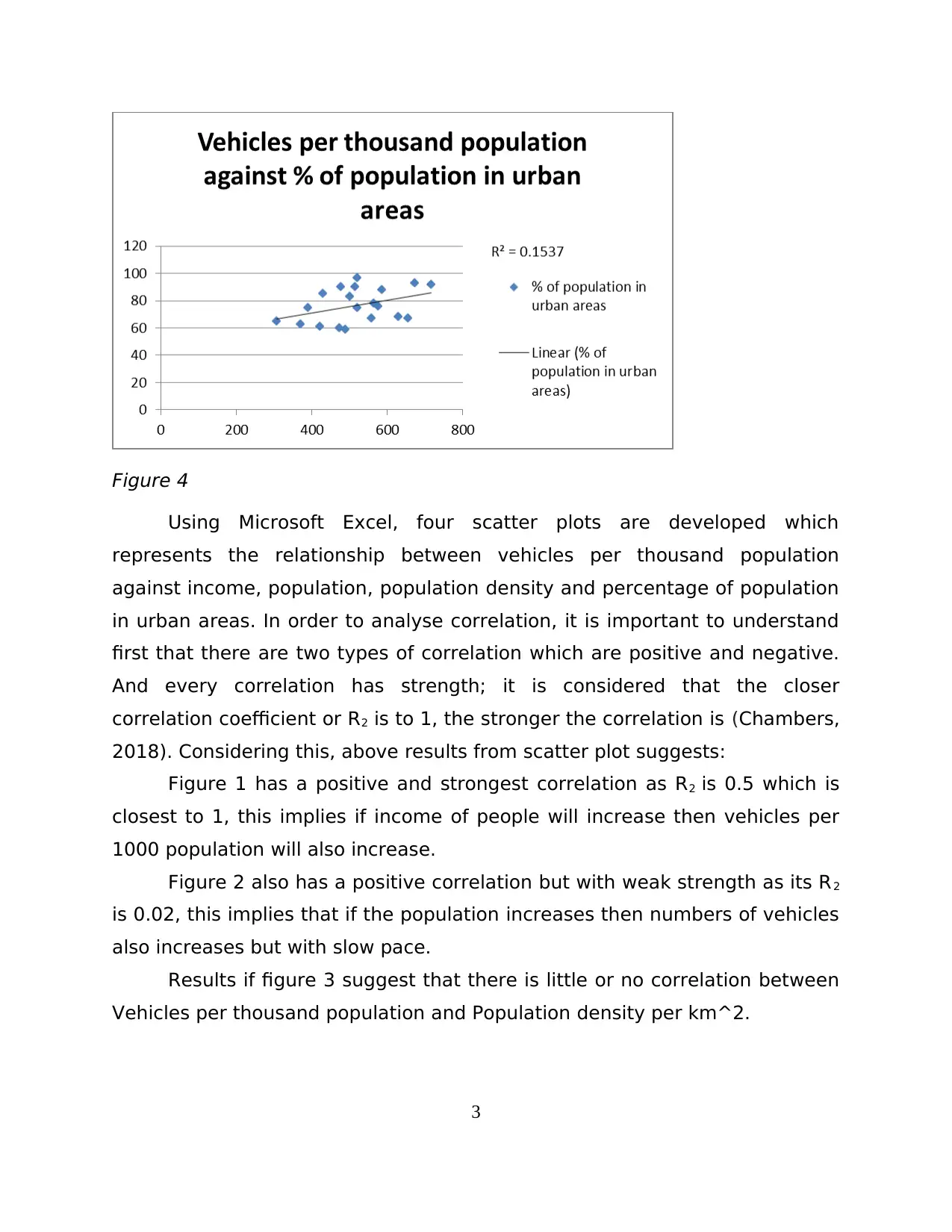
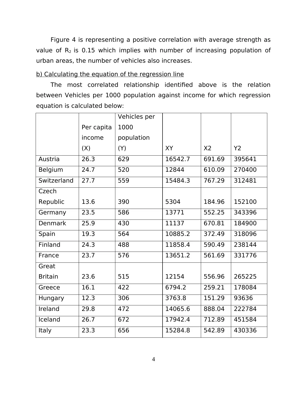
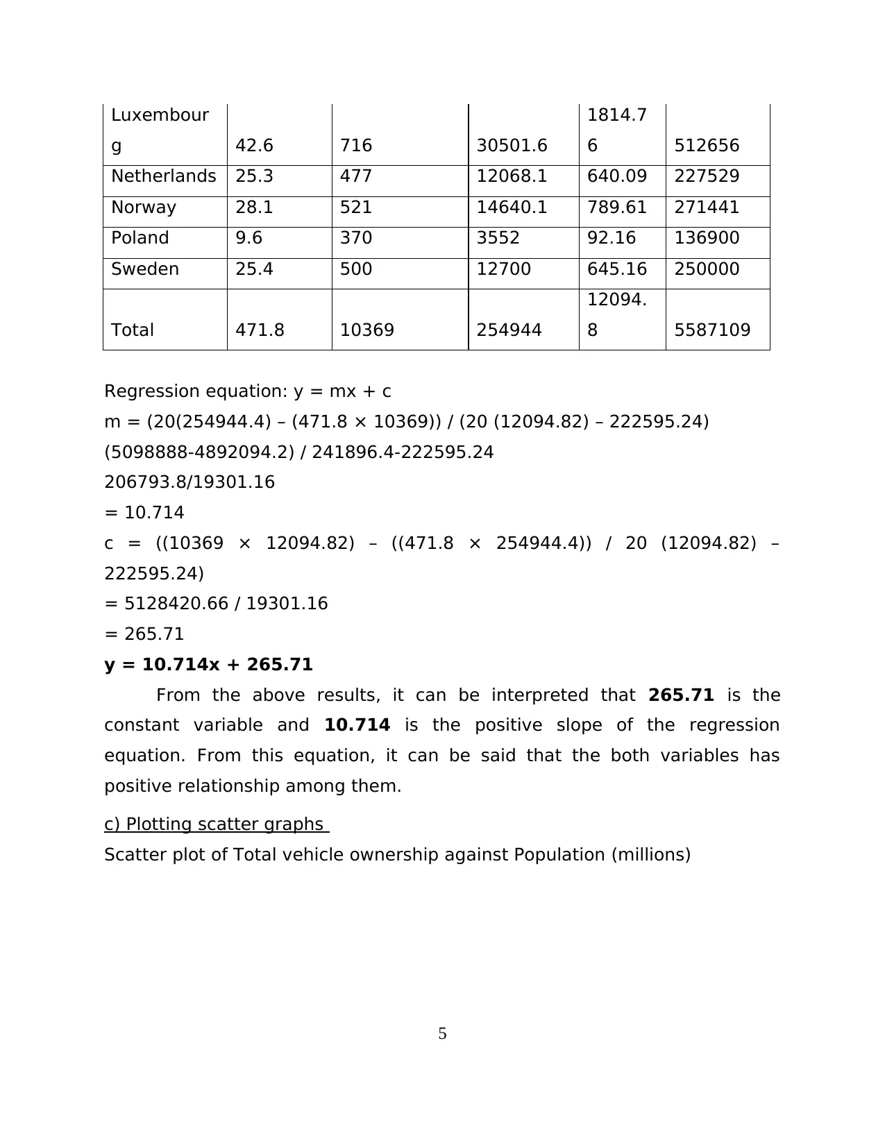
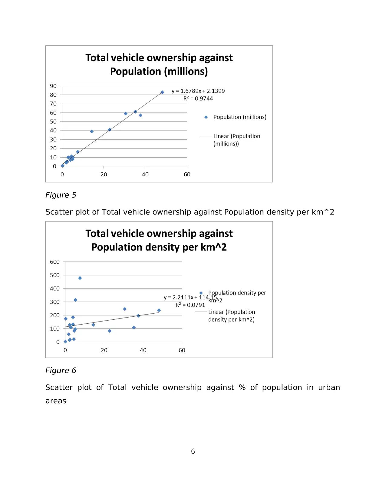
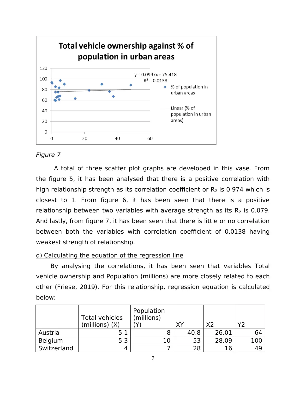
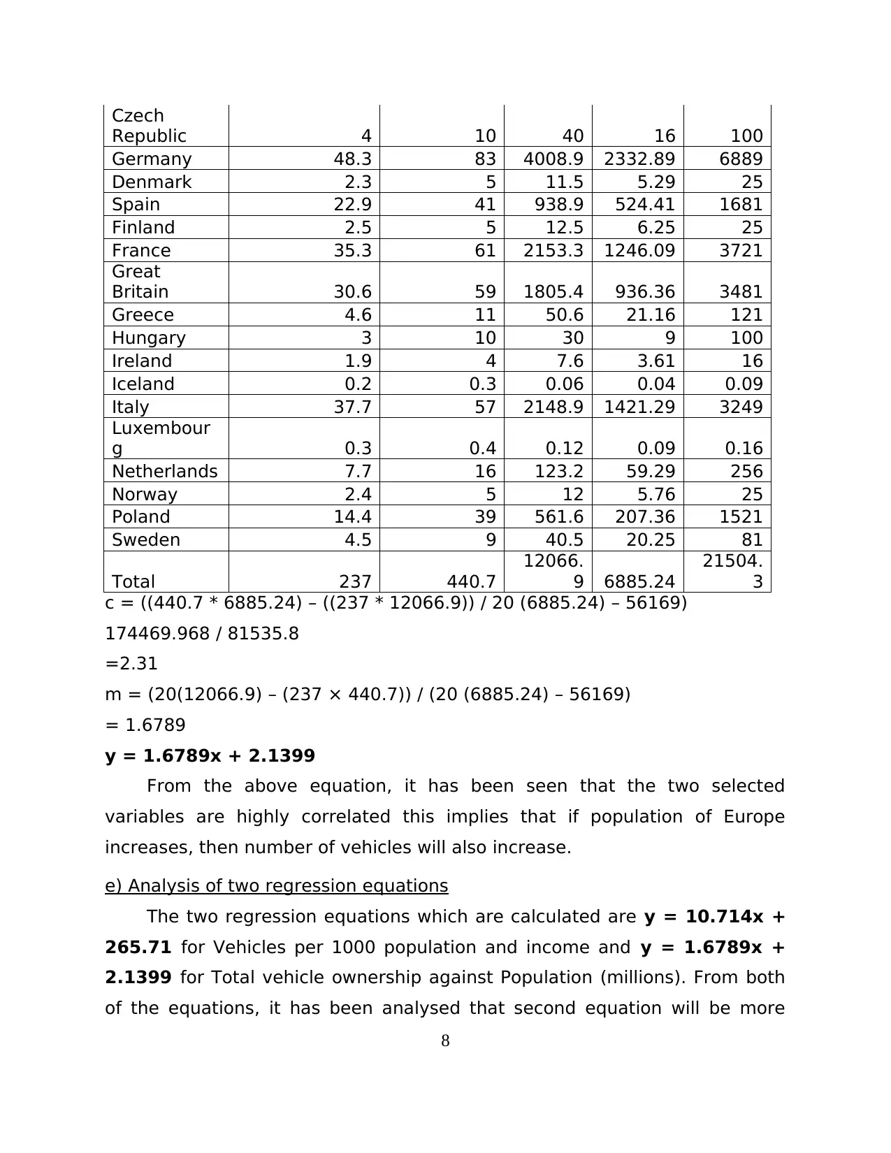
This report presents a data analysis of factors influencing vehicle ownership in European countries, prepared for AutoMobile Inc., a car distributor considering market expansion. The analysis employs scatter plots, regression, and correlation techniques to assess the relationships between vehicle ownership (per 1000 population and total ownership) and variables such as income, population, population density, and urbanization. Key findings include a strong positive correlation between income and vehicles per 1000 population, and between total vehicle ownership and population. Regression equations are calculated to model these relationships, with the equation for total vehicle ownership against population deemed more useful for AutoMobile Inc. The report also includes an analysis of data from Turkey, comparing predicted and actual vehicle ownership figures, and concludes that data analysis is crucial for effective decision-making, suggesting that AutoMobile Inc. should consider expanding into Turkey.

Business Statistics
and Data Analysis

ABSTRACT
This report is a summarisation of data analysis technique. A
manufacturing firm is considered in this report which is considering
expanding its operations. Scatter plots, regression and correlation are used
in order to suggest the appropriate direction to this company.

Contents
ABSTRACT........................................................................................................2
INTRODUCTION................................................................................................1
MAIN BODY......................................................................................................1
a) Plotting scatter graphs and analysing results for correlation...................1
b) Calculating the equation of the regression line........................................4
c) Plotting scatter graphs.............................................................................5
d) Calculating the equation of the regression line........................................7
e) Analysis of two regression equations.......................................................8
f) Data analysis of Turkey data.....................................................................8
CONCLUSION...................................................................................................8
REFERENCES....................................................................................................9

INTRODUCTION
Business statistics is the field of study in which data information is used
for effective decisions in a business (Bhunia, 2013). This concept is related
with Data Analysis which refers to the procedure of analysing the data using
numerical and graphical methods (Dixon and Woolner, 2012). The main aim
of this report is to build an understanding about data analysis procedure
using scatter plots. For this purpose, a scenario is given according to which a
car distributor firm AutoMobile Inc. is considering to expand in new market.
This decision is analysed using scatter plots and correlation methods in this
report.
MAIN BODY
a) Plotting scatter graphs and analysing results for correlation
Scatter graph for Vehicles per 1000 population against income
Figure 1
Scatter graph for Vehicles per 1000 population against Population (millions)
1

Figure 2
Scatter graph for Vehicles per 1000 population against Population density
per km^2
Figure 3
Scatter graph for Vehicles per 1000 population against % of population in
urban areas
2

Figure 4
Using Microsoft Excel, four scatter plots are developed which
represents the relationship between vehicles per thousand population
against income, population, population density and percentage of population
in urban areas. In order to analyse correlation, it is important to understand
first that there are two types of correlation which are positive and negative.
And every correlation has strength; it is considered that the closer
correlation coefficient or R2 is to 1, the stronger the correlation is (Chambers,
2018). Considering this, above results from scatter plot suggests:
Figure 1 has a positive and strongest correlation as R2 is 0.5 which is
closest to 1, this implies if income of people will increase then vehicles per
1000 population will also increase.
Figure 2 also has a positive correlation but with weak strength as its R2
is 0.02, this implies that if the population increases then numbers of vehicles
also increases but with slow pace.
Results if figure 3 suggest that there is little or no correlation between
Vehicles per thousand population and Population density per km^2.
3

Figure 4 is representing a positive correlation with average strength as
value of R2 is 0.15 which implies with number of increasing population of
urban areas, the number of vehicles also increases.
b) Calculating the equation of the regression line
The most correlated relationship identified above is the relation
between Vehicles per 1000 population against income for which regression
equation is calculated below:
Per capita
income
(X)
Vehicles per
1000
population
(Y) XY X2 Y2
Austria 26.3 629 16542.7 691.69 395641
Belgium 24.7 520 12844 610.09 270400
Switzerland 27.7 559 15484.3 767.29 312481
Czech
Republic 13.6 390 5304 184.96 152100
Germany 23.5 586 13771 552.25 343396
Denmark 25.9 430 11137 670.81 184900
Spain 19.3 564 10885.2 372.49 318096
Finland 24.3 488 11858.4 590.49 238144
France 23.7 576 13651.2 561.69 331776
Great
Britain 23.6 515 12154 556.96 265225
Greece 16.1 422 6794.2 259.21 178084
Hungary 12.3 306 3763.8 151.29 93636
Ireland 29.8 472 14065.6 888.04 222784
Iceland 26.7 672 17942.4 712.89 451584
Italy 23.3 656 15284.8 542.89 430336
4

Luxembour
g 42.6 716 30501.6
1814.7
6 512656
Netherlands 25.3 477 12068.1 640.09 227529
Norway 28.1 521 14640.1 789.61 271441
Poland 9.6 370 3552 92.16 136900
Sweden 25.4 500 12700 645.16 250000
Total 471.8 10369 254944
12094.
8 5587109
Regression equation: y = mx + c
m = (20(254944.4) – (471.8 × 10369)) / (20 (12094.82) – 222595.24)
(5098888-4892094.2) / 241896.4-222595.24
206793.8/19301.16
= 10.714
c = ((10369 × 12094.82) – ((471.8 × 254944.4)) / 20 (12094.82) –
222595.24)
= 5128420.66 / 19301.16
= 265.71
y = 10.714x + 265.71
From the above results, it can be interpreted that 265.71 is the
constant variable and 10.714 is the positive slope of the regression
equation. From this equation, it can be said that the both variables has
positive relationship among them.
c) Plotting scatter graphs
Scatter plot of Total vehicle ownership against Population (millions)
5

Figure 5
Scatter plot of Total vehicle ownership against Population density per km^2
Figure 6
Scatter plot of Total vehicle ownership against % of population in urban
areas
6

Figure 7
A total of three scatter plot graphs are developed in this vase. From
the figure 5, it has been analysed that there is a positive correlation with
high relationship strength as its correlation coefficient or R2 is 0.974 which is
closest to 1. From figure 6, it has been seen that there is a positive
relationship between two variables with average strength as its R2 is 0.079.
And lastly, from figure 7, it has been seen that there is little or no correlation
between both the variables with correlation coefficient of 0.0138 having
weakest strength of relationship.
d) Calculating the equation of the regression line
By analysing the correlations, it has been seen that variables Total
vehicle ownership and Population (millions) are more closely related to each
other (Friese, 2019). For this relationship, regression equation is calculated
below:
Total vehicles
(millions) (X)
Population
(millions)
(Y) XY X2 Y2
Austria 5.1 8 40.8 26.01 64
Belgium 5.3 10 53 28.09 100
Switzerland 4 7 28 16 49
7

Czech
Republic 4 10 40 16 100
Germany 48.3 83 4008.9 2332.89 6889
Denmark 2.3 5 11.5 5.29 25
Spain 22.9 41 938.9 524.41 1681
Finland 2.5 5 12.5 6.25 25
France 35.3 61 2153.3 1246.09 3721
Great
Britain 30.6 59 1805.4 936.36 3481
Greece 4.6 11 50.6 21.16 121
Hungary 3 10 30 9 100
Ireland 1.9 4 7.6 3.61 16
Iceland 0.2 0.3 0.06 0.04 0.09
Italy 37.7 57 2148.9 1421.29 3249
Luxembour
g 0.3 0.4 0.12 0.09 0.16
Netherlands 7.7 16 123.2 59.29 256
Norway 2.4 5 12 5.76 25
Poland 14.4 39 561.6 207.36 1521
Sweden 4.5 9 40.5 20.25 81
Total 237 440.7
12066.
9 6885.24
21504.
3
c = ((440.7 * 6885.24) – ((237 * 12066.9)) / 20 (6885.24) – 56169)
174469.968 / 81535.8
=2.31
m = (20(12066.9) – (237 × 440.7)) / (20 (6885.24) – 56169)
= 1.6789
y = 1.6789x + 2.1399
From the above equation, it has been seen that the two selected
variables are highly correlated this implies that if population of Europe
increases, then number of vehicles will also increase.
e) Analysis of two regression equations
The two regression equations which are calculated are y = 10.714x +
265.71 for Vehicles per 1000 population and income and y = 1.6789x +
2.1399 for Total vehicle ownership against Population (millions). From both
of the equations, it has been analysed that second equation will be more
8

useful for AutoMobile Inc. as second equation has high strength of correlation
with coefficient of 0.97 which is more closer to 1 (Ghilani, 2017).
f) Data analysis of Turkey data
Using the data for Turkey and regression equation of “y = 10.714x +
265.71”, Vehicles per 1000 population for Turkey is calculated as 331 which
is different from actual results of 96.
On the other hand, using Turkey data and regression equation of “y =
1.6789x + 2.1399” Total vehicles in millions are calculated as 37.94 million
which is different from its actual result of 6.4 million.
The reason behind this difference is that regression equations and
predictions are done using certain set of formula which is y = mx + c in this
case which can be different from the actual results. The predictions are
made by using pats information and it does not consider any external
environmental factors (Wang, Chiou and Müller, 2016).
CONCLUSION
From the above report, it has been analysed that data analysis can be
used by an organisation for the purpose of effective decision making. The
AutoMobile firm should consider in expanding into Turkey as it can gain
higher prospects.
9

REFERENCES
Books and Journals
Bhunia, A., 2013. Statistical methods for practice and research (A guide to
data analysis using SPSS). South Asian Journal of Management. 20(1).
154.
Chambers, J.M., 2018. Graphical methods for data analysis. CRC Press.
Dixon, P., and Woolner, P., 2012. Quantitative data analysis: using
SPSS. Research methods in educational leadership and management,
340.
Friese, S., 2019. Qualitative data analysis with ATLAS. ti. SAGE Publications
Limited.
Ghilani, C.D., 2017. Adjustment computations: spatial data analysis. John
Wiley & Sons.
Wang, J.L., Chiou, J.M. and Müller, H.G., 2016. Functional data analysis.
Annual Review of Statistics and Its Application, 3, pp.257-295.
10