BAC115 Quantitative Methods: Service Time Analysis at Gourmet Delight
VerifiedAdded on 2023/06/04
|12
|2347
|318
Report
AI Summary
This report presents a quantitative analysis of service times at Gourmet Delight, a five-star restaurant in Melbourne, before and after staff training, as well as six months post-training. The analysis includes descriptive statistics, boxplots, and histograms to compare service times. Regression analysis is used to assess the impact of advertising expenditure on monthly revenue, and exponential smoothing is applied to analyze patronage patterns. Trend analysis is performed to forecast restaurant takings, providing insights into the restaurant's performance and the effectiveness of implemented strategies. This document is a valuable resource for students, and Desklib provides access to similar solved assignments and study tools.

Running Head: SERVING TIME ANALYSIS – QUANTITATIVE RESEARCH
Serving Time Analysis – Quantitative Research
Name of the Student
Name of the University
Author Note
Serving Time Analysis – Quantitative Research
Name of the Student
Name of the University
Author Note
Paraphrase This Document
Need a fresh take? Get an instant paraphrase of this document with our AI Paraphraser
1SERVING TIME ANALYSIS – QUANTITATIVE RESEARCH
Table of Contents
Part A – Service Time Analysis.......................................................................................................2
Service Times before and After Training....................................................................................2
Service Times 6 Months after Training.......................................................................................5
Part B – Patronage to Gourmet Delight...........................................................................................7
Part C – Patronage Pattern and Restaurant Takings........................................................................8
Patronage Pattern.........................................................................................................................8
Restaurant Takings......................................................................................................................9
2SERVING TIME ANALYSIS – QUANTITATIVE RESEARCH
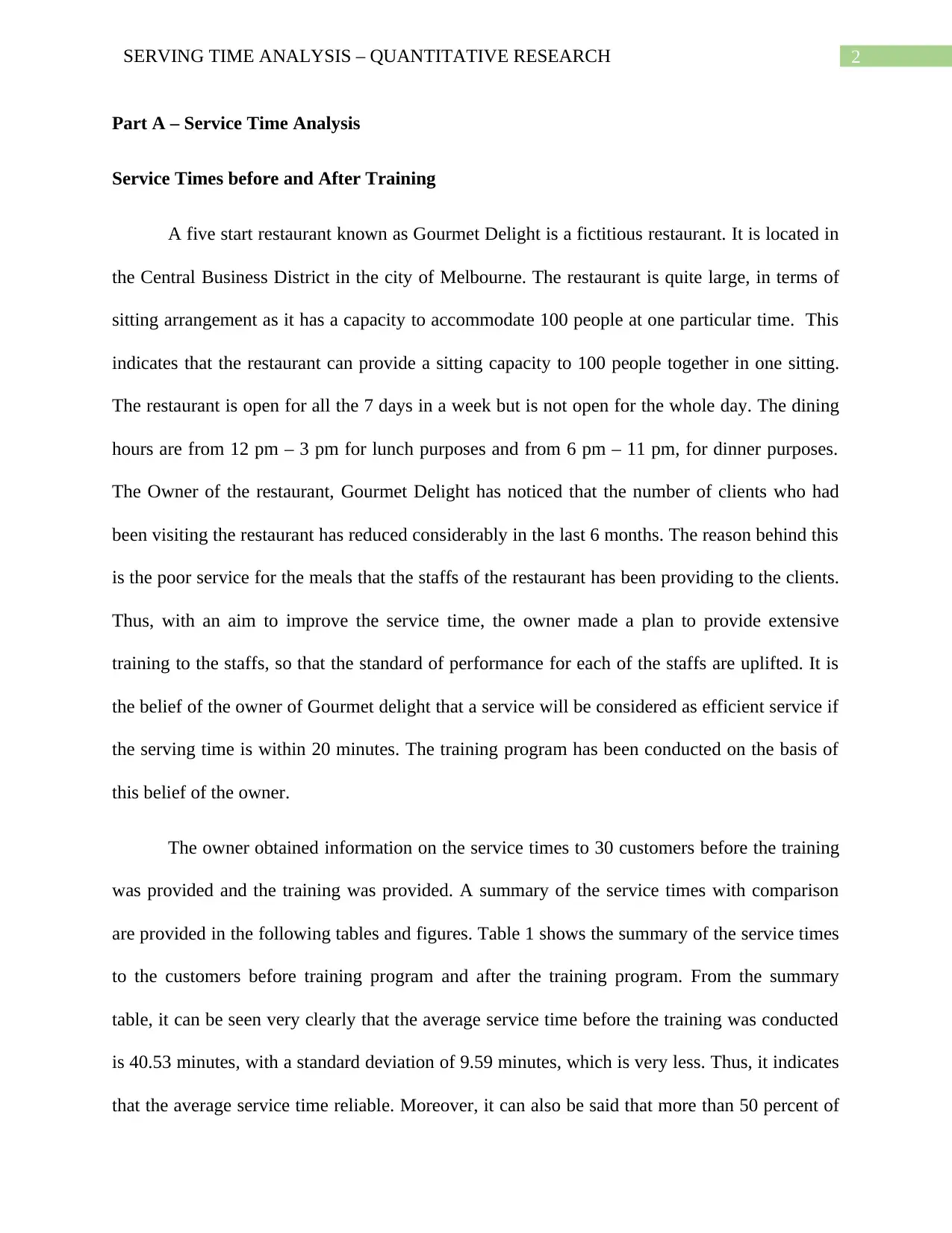
Part A – Service Time Analysis
Service Times before and After Training
A five start restaurant known as Gourmet Delight is a fictitious restaurant. It is located in
the Central Business District in the city of Melbourne. The restaurant is quite large, in terms of
sitting arrangement as it has a capacity to accommodate 100 people at one particular time. This
indicates that the restaurant can provide a sitting capacity to 100 people together in one sitting.
The restaurant is open for all the 7 days in a week but is not open for the whole day. The dining
hours are from 12 pm – 3 pm for lunch purposes and from 6 pm – 11 pm, for dinner purposes.
The Owner of the restaurant, Gourmet Delight has noticed that the number of clients who had
been visiting the restaurant has reduced considerably in the last 6 months. The reason behind this
is the poor service for the meals that the staffs of the restaurant has been providing to the clients.
Thus, with an aim to improve the service time, the owner made a plan to provide extensive
training to the staffs, so that the standard of performance for each of the staffs are uplifted. It is
the belief of the owner of Gourmet delight that a service will be considered as efficient service if
the serving time is within 20 minutes. The training program has been conducted on the basis of
this belief of the owner.
The owner obtained information on the service times to 30 customers before the training
was provided and the training was provided. A summary of the service times with comparison
are provided in the following tables and figures. Table 1 shows the summary of the service times
to the customers before training program and after the training program. From the summary
table, it can be seen very clearly that the average service time before the training was conducted
is 40.53 minutes, with a standard deviation of 9.59 minutes, which is very less. Thus, it indicates
that the average service time reliable. Moreover, it can also be said that more than 50 percent of
⊘ This is a preview!⊘
Do you want full access?
Subscribe today to unlock all pages.
Trusted by 1+ million students worldwide
3SERVING TIME ANALYSIS – QUANTITATIVE RESEARCH
the clients have been served food in a time higher than 39.5 minutes. Thus, the clients were not
at all provided with efficient services. Hence, the loss in the number of clientele. On the other
hand, from the analysis of the service times after training, it can be seen that the average service
time has reduced to 20 minutes, with a standard deviation of 6.65 minutes, which is less. Thus, it
indicates that the average service time reliable. Moreover, it can also be said that less than 50
percent of the clients have been served food in a time less than 19 minutes and no customers
have been found to be served in a time higher than 34 minutes. Thus, the clients were mostly
provided with efficient services.
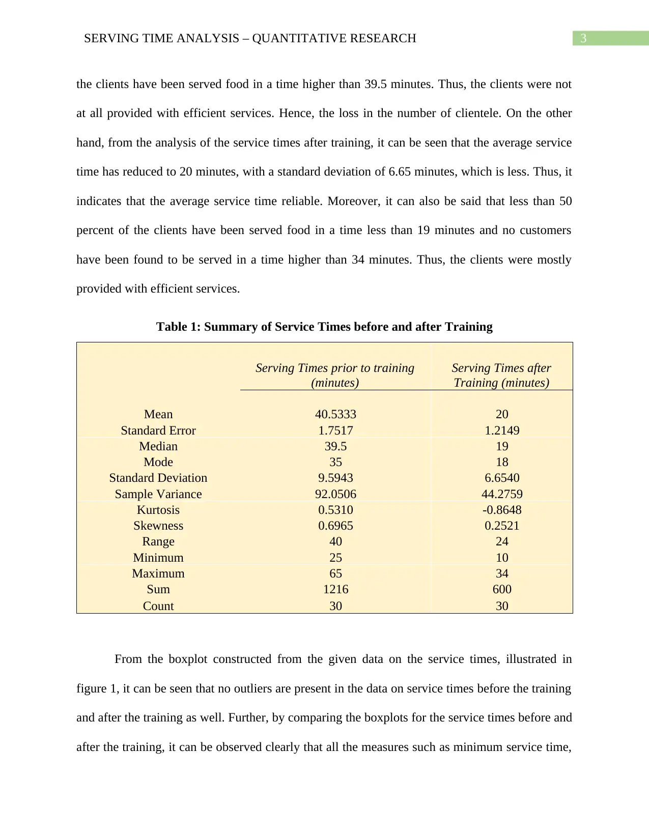
Table 1: Summary of Service Times before and after Training
Serving Times prior to training
(minutes)
Serving Times after
Training (minutes)
Mean 40.5333 20
Standard Error 1.7517 1.2149
Median 39.5 19
Mode 35 18
Standard Deviation 9.5943 6.6540
Sample Variance 92.0506 44.2759
Kurtosis 0.5310 -0.8648
Skewness 0.6965 0.2521
Range 40 24
Minimum 25 10
Maximum 65 34
Sum 1216 600
Count 30 30
From the boxplot constructed from the given data on the service times, illustrated in
figure 1, it can be seen that no outliers are present in the data on service times before the training
and after the training as well. Further, by comparing the boxplots for the service times before and
after the training, it can be observed clearly that all the measures such as minimum service time,
the clients have been served food in a time higher than 39.5 minutes. Thus, the clients were not
at all provided with efficient services. Hence, the loss in the number of clientele. On the other
hand, from the analysis of the service times after training, it can be seen that the average service
time has reduced to 20 minutes, with a standard deviation of 6.65 minutes, which is less. Thus, it
indicates that the average service time reliable. Moreover, it can also be said that less than 50
percent of the clients have been served food in a time less than 19 minutes and no customers
have been found to be served in a time higher than 34 minutes. Thus, the clients were mostly
provided with efficient services.
Table 1: Summary of Service Times before and after Training
Serving Times prior to training
(minutes)
Serving Times after
Training (minutes)
Mean 40.5333 20
Standard Error 1.7517 1.2149
Median 39.5 19
Mode 35 18
Standard Deviation 9.5943 6.6540
Sample Variance 92.0506 44.2759
Kurtosis 0.5310 -0.8648
Skewness 0.6965 0.2521
Range 40 24
Minimum 25 10
Maximum 65 34
Sum 1216 600
Count 30 30
From the boxplot constructed from the given data on the service times, illustrated in
figure 1, it can be seen that no outliers are present in the data on service times before the training
and after the training as well. Further, by comparing the boxplots for the service times before and
after the training, it can be observed clearly that all the measures such as minimum service time,
Paraphrase This Document
Need a fresh take? Get an instant paraphrase of this document with our AI Paraphraser

4SERVING TIME ANALYSIS – QUANTITATIVE RESEARCH
first quartile (indicating the least 25 percent of the service times), third quartile (indicating the
least 75 percent of the service times) and the maximum service time are higher before the
training was provided than after the training.
0 10 20 30 40 50 60 70
Serving Times
after Training
(minutes)
Serving Times
prior to training
(minutes)
Boxplot
Figure 1: Boxplot Comparing serving times before and after Training
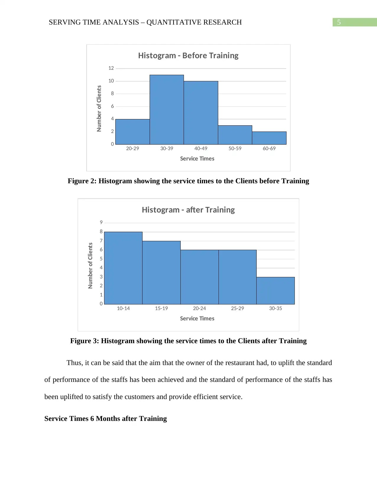
Further, from the histograms comparing the service times to the clients before and after
the training program, given in figures 2 and 3 respectively, it can be seen that the distribution of
the service times before and after the training are approximately normal. The mean or average is
said to be the best measure of central tendency for a normal distribution and hence, it can be said
that the average serving time after the training has reduced from that before the training.
first quartile (indicating the least 25 percent of the service times), third quartile (indicating the
least 75 percent of the service times) and the maximum service time are higher before the
training was provided than after the training.
0 10 20 30 40 50 60 70
Serving Times
after Training
(minutes)
Serving Times
prior to training
(minutes)
Boxplot
Figure 1: Boxplot Comparing serving times before and after Training
Further, from the histograms comparing the service times to the clients before and after
the training program, given in figures 2 and 3 respectively, it can be seen that the distribution of
the service times before and after the training are approximately normal. The mean or average is
said to be the best measure of central tendency for a normal distribution and hence, it can be said
that the average serving time after the training has reduced from that before the training.
5SERVING TIME ANALYSIS – QUANTITATIVE RESEARCH
20-29 30-39 40-49 50-59 60-69
0
2
4
6
8
10
12
Histogram - Before Training
Service Times
Number of Clients
Figure 2: Histogram showing the service times to the Clients before Training
10-14 15-19 20-24 25-29 30-35
0
1
2
3
4
5
6
7
8
9
Histogram - after Training
Service Times
Number of Clients
Figure 3: Histogram showing the service times to the Clients after Training
Thus, it can be said that the aim that the owner of the restaurant had, to uplift the standard
of performance of the staffs has been achieved and the standard of performance of the staffs has
been uplifted to satisfy the customers and provide efficient service.
Service Times 6 Months after Training
⊘ This is a preview!⊘
Do you want full access?
Subscribe today to unlock all pages.
Trusted by 1+ million students worldwide
6SERVING TIME ANALYSIS – QUANTITATIVE RESEARCH
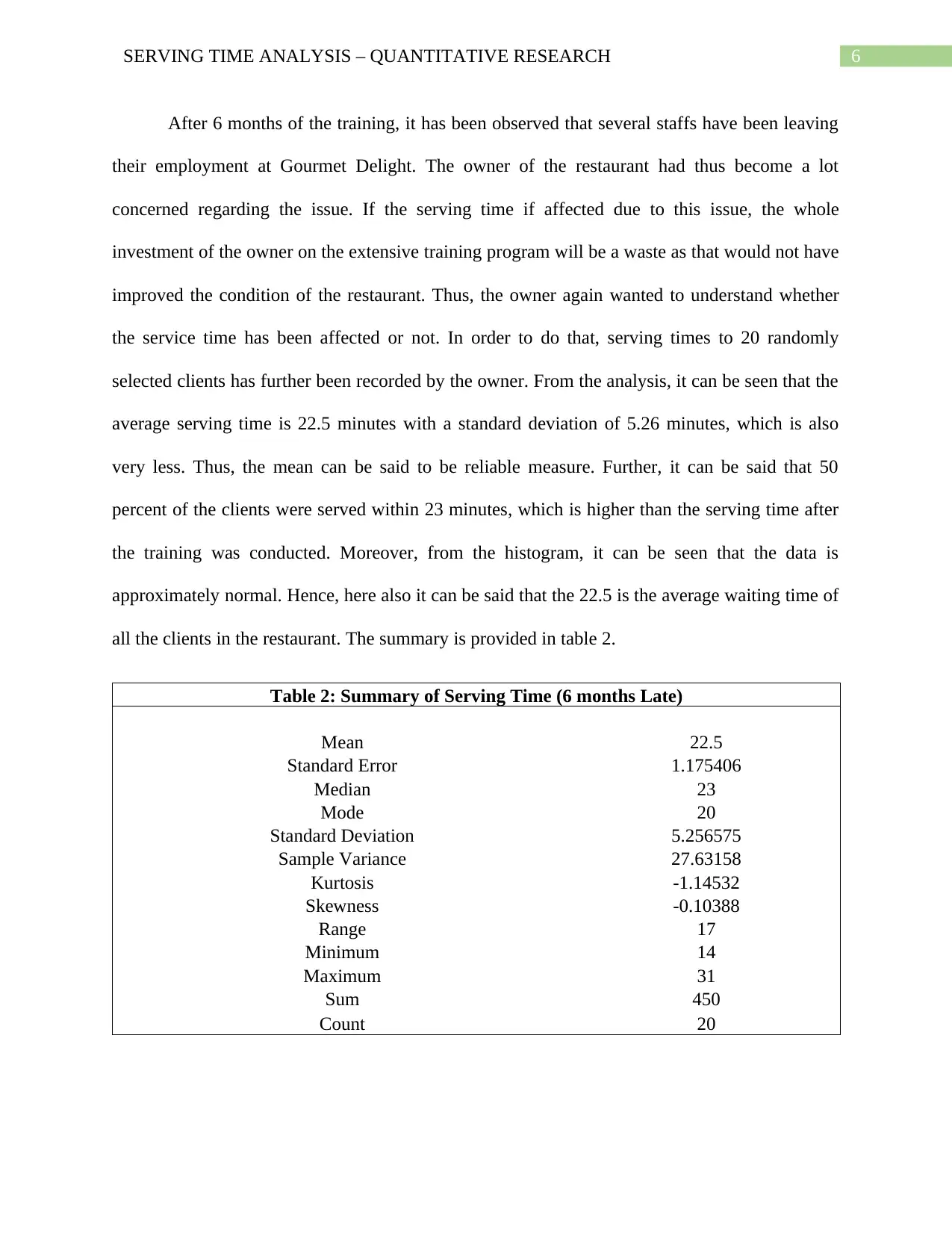
After 6 months of the training, it has been observed that several staffs have been leaving
their employment at Gourmet Delight. The owner of the restaurant had thus become a lot
concerned regarding the issue. If the serving time if affected due to this issue, the whole
investment of the owner on the extensive training program will be a waste as that would not have
improved the condition of the restaurant. Thus, the owner again wanted to understand whether
the service time has been affected or not. In order to do that, serving times to 20 randomly
selected clients has further been recorded by the owner. From the analysis, it can be seen that the
average serving time is 22.5 minutes with a standard deviation of 5.26 minutes, which is also
very less. Thus, the mean can be said to be reliable measure. Further, it can be said that 50
percent of the clients were served within 23 minutes, which is higher than the serving time after
the training was conducted. Moreover, from the histogram, it can be seen that the data is
approximately normal. Hence, here also it can be said that the 22.5 is the average waiting time of
all the clients in the restaurant. The summary is provided in table 2.
Table 2: Summary of Serving Time (6 months Late)
Mean 22.5
Standard Error 1.175406
Median 23
Mode 20
Standard Deviation 5.256575
Sample Variance 27.63158
Kurtosis -1.14532
Skewness -0.10388
Range 17
Minimum 14
Maximum 31
Sum 450
Count 20
Paraphrase This Document
Need a fresh take? Get an instant paraphrase of this document with our AI Paraphraser
7SERVING TIME ANALYSIS – QUANTITATIVE RESEARCH
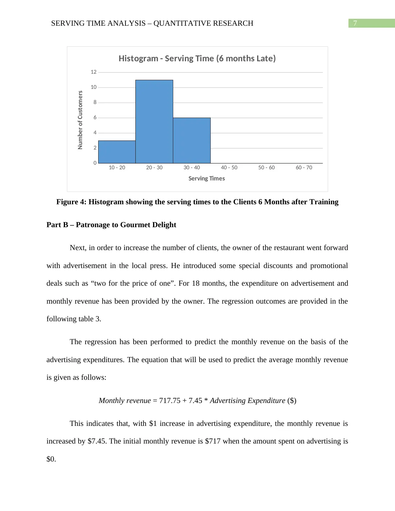
10 - 20 20 - 30 30 - 40 40 - 50 50 - 60 60 - 70
0
2
4
6
8
10
12
Histogram - Serving Time (6 months Late)
Serving Times
Number of Customers
Figure 4: Histogram showing the serving times to the Clients 6 Months after Training
Part B – Patronage to Gourmet Delight
Next, in order to increase the number of clients, the owner of the restaurant went forward
with advertisement in the local press. He introduced some special discounts and promotional
deals such as “two for the price of one”. For 18 months, the expenditure on advertisement and
monthly revenue has been provided by the owner. The regression outcomes are provided in the
following table 3.
The regression has been performed to predict the monthly revenue on the basis of the
advertising expenditures. The equation that will be used to predict the average monthly revenue
is given as follows:
Monthly revenue = 717.75 + 7.45 * Advertising Expenditure ($)
This indicates that, with $1 increase in advertising expenditure, the monthly revenue is
increased by $7.45. The initial monthly revenue is $717 when the amount spent on advertising is
$0.
8SERVING TIME ANALYSIS – QUANTITATIVE RESEARCH
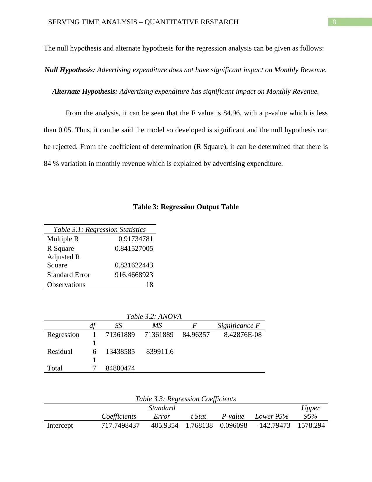
The null hypothesis and alternate hypothesis for the regression analysis can be given as follows:
Null Hypothesis: Advertising expenditure does not have significant impact on Monthly Revenue.
Alternate Hypothesis: Advertising expenditure has significant impact on Monthly Revenue.
From the analysis, it can be seen that the F value is 84.96, with a p-value which is less
than 0.05. Thus, it can be said the model so developed is significant and the null hypothesis can
be rejected. From the coefficient of determination (R Square), it can be determined that there is
84 % variation in monthly revenue which is explained by advertising expenditure.
Table 3: Regression Output Table
Table 3.1: Regression Statistics
Multiple R 0.91734781
R Square 0.841527005
Adjusted R
Square 0.831622443
Standard Error 916.4668923
Observations 18
Table 3.2: ANOVA
df SS MS F Significance F
Regression 1 71361889 71361889 84.96357 8.42876E-08
Residual
1
6 13438585 839911.6
Total
1
7 84800474
Table 3.3: Regression Coefficients
Coefficients
Standard
Error t Stat P-value Lower 95%
Upper
95%
Intercept 717.7498437 405.9354 1.768138 0.096098 -142.79473 1578.294
⊘ This is a preview!⊘
Do you want full access?
Subscribe today to unlock all pages.
Trusted by 1+ million students worldwide
9SERVING TIME ANALYSIS – QUANTITATIVE RESEARCH
Advertising
Expenditure($) 7.449183908 0.808151 9.217569 8.43E-08 5.735981 9.162387
Part C – Patronage Pattern and Restaurant Takings
Patronage Pattern
The exponential smoothing to a given data series can be estimated with the help of the
following equation:
Exponential Smoothing (ES): Ft+ 1=Ft + a( At−Ft )
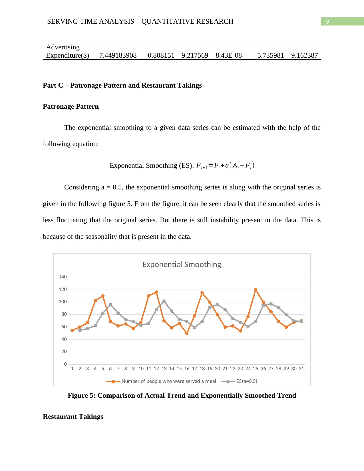
Considering a = 0.5, the exponential smoothing series is along with the original series is
given in the following figure 5. From the figure, it can be seen clearly that the smoothed series is
less fluctuating that the original series. But there is still instability present in the data. This is
because of the seasonality that is present in the data.
1 2 3 4 5 6 7 8 9 10 11 12 13 14 15 16 17 18 19 20 21 22 23 24 25 26 27 28 29 30 31
0
20
40
60
80
100
120
140
Exponential Smoothing
Number of people who were served a meal ES(a=0.5)
Figure 5: Comparison of Actual Trend and Exponentially Smoothed Trend
Restaurant Takings
Advertising
Expenditure($) 7.449183908 0.808151 9.217569 8.43E-08 5.735981 9.162387
Part C – Patronage Pattern and Restaurant Takings
Patronage Pattern
The exponential smoothing to a given data series can be estimated with the help of the
following equation:
Exponential Smoothing (ES): Ft+ 1=Ft + a( At−Ft )
Considering a = 0.5, the exponential smoothing series is along with the original series is
given in the following figure 5. From the figure, it can be seen clearly that the smoothed series is
less fluctuating that the original series. But there is still instability present in the data. This is
because of the seasonality that is present in the data.
1 2 3 4 5 6 7 8 9 10 11 12 13 14 15 16 17 18 19 20 21 22 23 24 25 26 27 28 29 30 31
0
20
40
60
80
100
120
140
Exponential Smoothing
Number of people who were served a meal ES(a=0.5)
Figure 5: Comparison of Actual Trend and Exponentially Smoothed Trend
Restaurant Takings
Paraphrase This Document
Need a fresh take? Get an instant paraphrase of this document with our AI Paraphraser
10SERVING TIME ANALYSIS – QUANTITATIVE RESEARCH
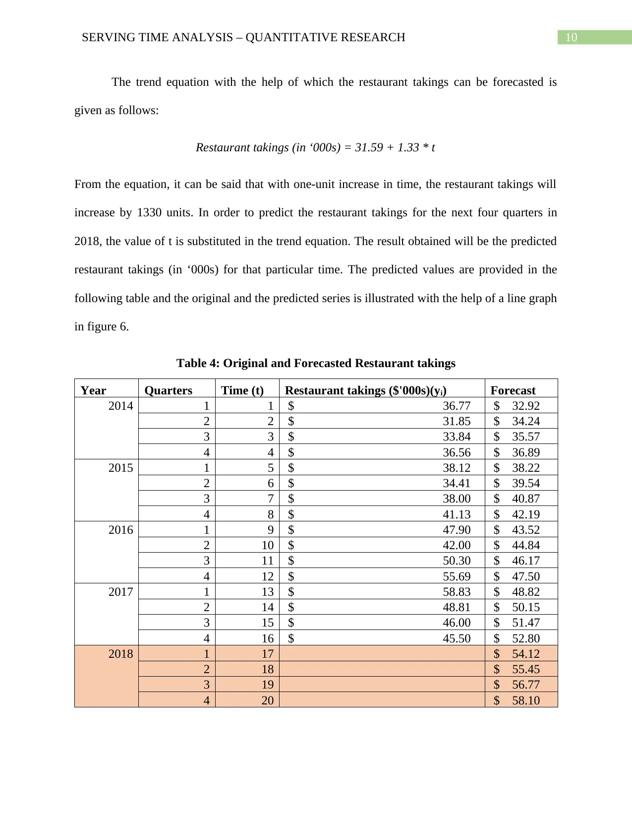
The trend equation with the help of which the restaurant takings can be forecasted is
given as follows:
Restaurant takings (in ‘000s) = 31.59 + 1.33 * t
From the equation, it can be said that with one-unit increase in time, the restaurant takings will
increase by 1330 units. In order to predict the restaurant takings for the next four quarters in
2018, the value of t is substituted in the trend equation. The result obtained will be the predicted
restaurant takings (in ‘000s) for that particular time. The predicted values are provided in the
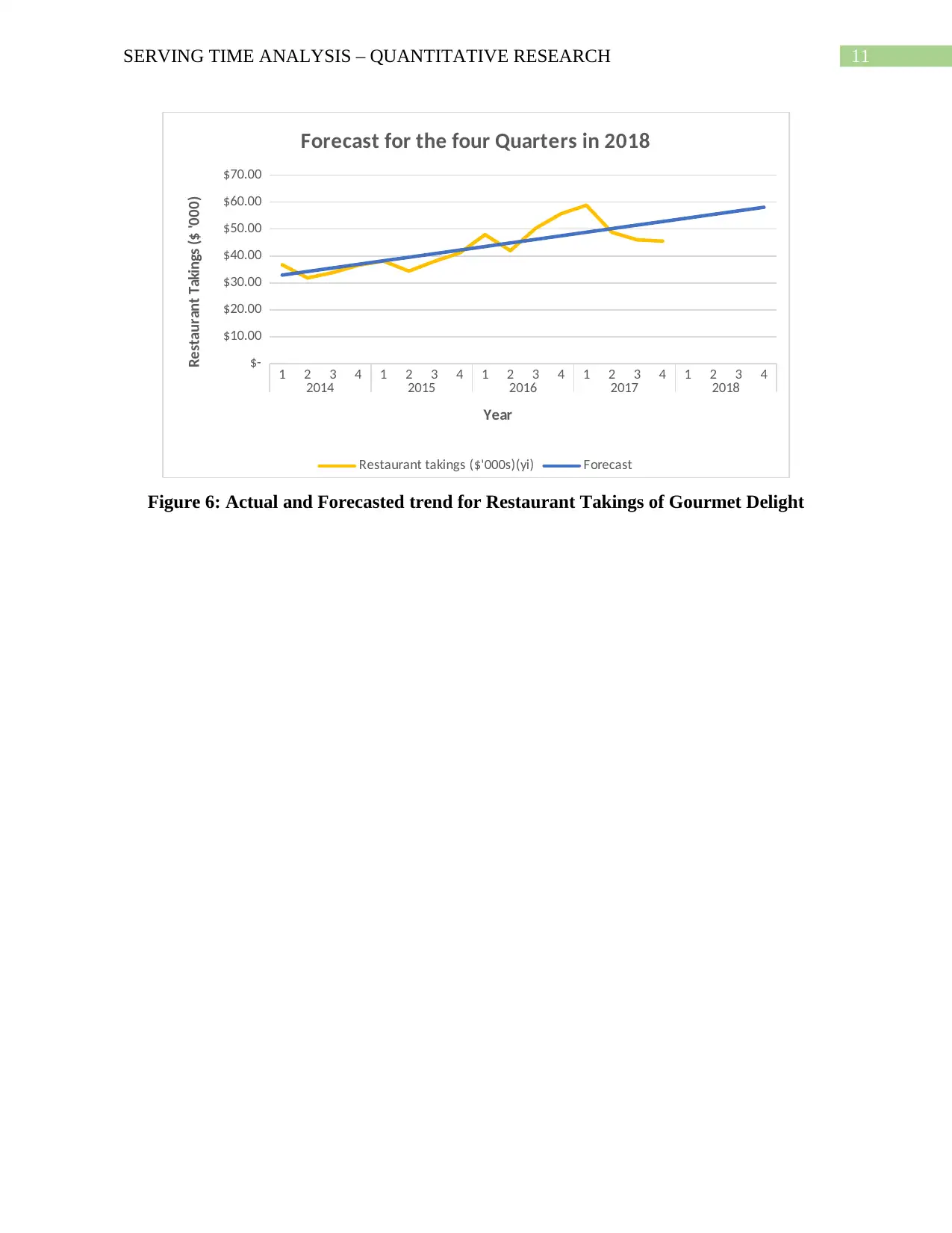
following table and the original and the predicted series is illustrated with the help of a line graph
in figure 6.
Table 4: Original and Forecasted Restaurant takings
Year Quarters Time (t) Restaurant takings ($'000s)(yi) Forecast
2014 1 1 $ 36.77 $ 32.92
2 2 $ 31.85 $ 34.24
3 3 $ 33.84 $ 35.57
4 4 $ 36.56 $ 36.89
2015 1 5 $ 38.12 $ 38.22
2 6 $ 34.41 $ 39.54
3 7 $ 38.00 $ 40.87
4 8 $ 41.13 $ 42.19
2016 1 9 $ 47.90 $ 43.52
2 10 $ 42.00 $ 44.84
3 11 $ 50.30 $ 46.17
4 12 $ 55.69 $ 47.50
2017 1 13 $ 58.83 $ 48.82
2 14 $ 48.81 $ 50.15
3 15 $ 46.00 $ 51.47
4 16 $ 45.50 $ 52.80
2018 1 17 $ 54.12
2 18 $ 55.45
3 19 $ 56.77
4 20 $ 58.10
The trend equation with the help of which the restaurant takings can be forecasted is
given as follows:
Restaurant takings (in ‘000s) = 31.59 + 1.33 * t
From the equation, it can be said that with one-unit increase in time, the restaurant takings will
increase by 1330 units. In order to predict the restaurant takings for the next four quarters in
2018, the value of t is substituted in the trend equation. The result obtained will be the predicted
restaurant takings (in ‘000s) for that particular time. The predicted values are provided in the
following table and the original and the predicted series is illustrated with the help of a line graph
in figure 6.
Table 4: Original and Forecasted Restaurant takings
Year Quarters Time (t) Restaurant takings ($'000s)(yi) Forecast
2014 1 1 $ 36.77 $ 32.92
2 2 $ 31.85 $ 34.24
3 3 $ 33.84 $ 35.57
4 4 $ 36.56 $ 36.89
2015 1 5 $ 38.12 $ 38.22
2 6 $ 34.41 $ 39.54
3 7 $ 38.00 $ 40.87
4 8 $ 41.13 $ 42.19
2016 1 9 $ 47.90 $ 43.52
2 10 $ 42.00 $ 44.84
3 11 $ 50.30 $ 46.17
4 12 $ 55.69 $ 47.50
2017 1 13 $ 58.83 $ 48.82
2 14 $ 48.81 $ 50.15
3 15 $ 46.00 $ 51.47
4 16 $ 45.50 $ 52.80
2018 1 17 $ 54.12
2 18 $ 55.45
3 19 $ 56.77
4 20 $ 58.10
11SERVING TIME ANALYSIS – QUANTITATIVE RESEARCH
1 2 3 4 1 2 3 4 1 2 3 4 1 2 3 4 1 2 3 4
2014 2015 2016 2017 2018
$-
$10.00
$20.00
$30.00
$40.00
$50.00
$60.00
$70.00
Forecast for the four Quarters in 2018
Restaurant takings ($'000s)(yi) Forecast
Year
Restaurant Takings ($ '000)
Figure 6: Actual and Forecasted trend for Restaurant Takings of Gourmet Delight
⊘ This is a preview!⊘
Do you want full access?
Subscribe today to unlock all pages.
Trusted by 1+ million students worldwide
1 out of 12
Related Documents


Your All-in-One AI-Powered Toolkit for Academic Success.
+13062052269
info@desklib.com
Available 24*7 on WhatsApp / Email
![[object Object]](/_next/static/media/star-bottom.7253800d.svg)
Unlock your academic potential
Copyright © 2020–2026 A2Z Services. All Rights Reserved. Developed and managed by ZUCOL.