Bayesian Estimation, Rao-Blackwell, and Statistical Inference

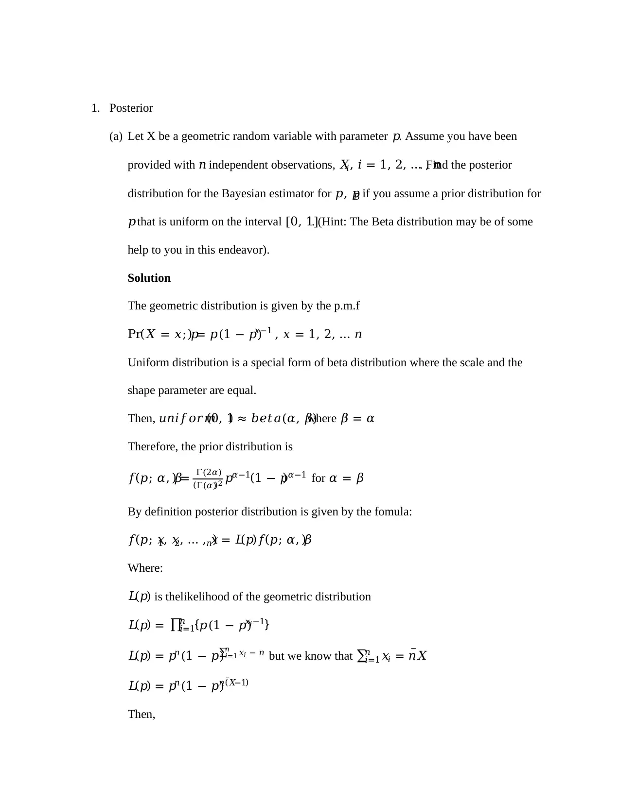
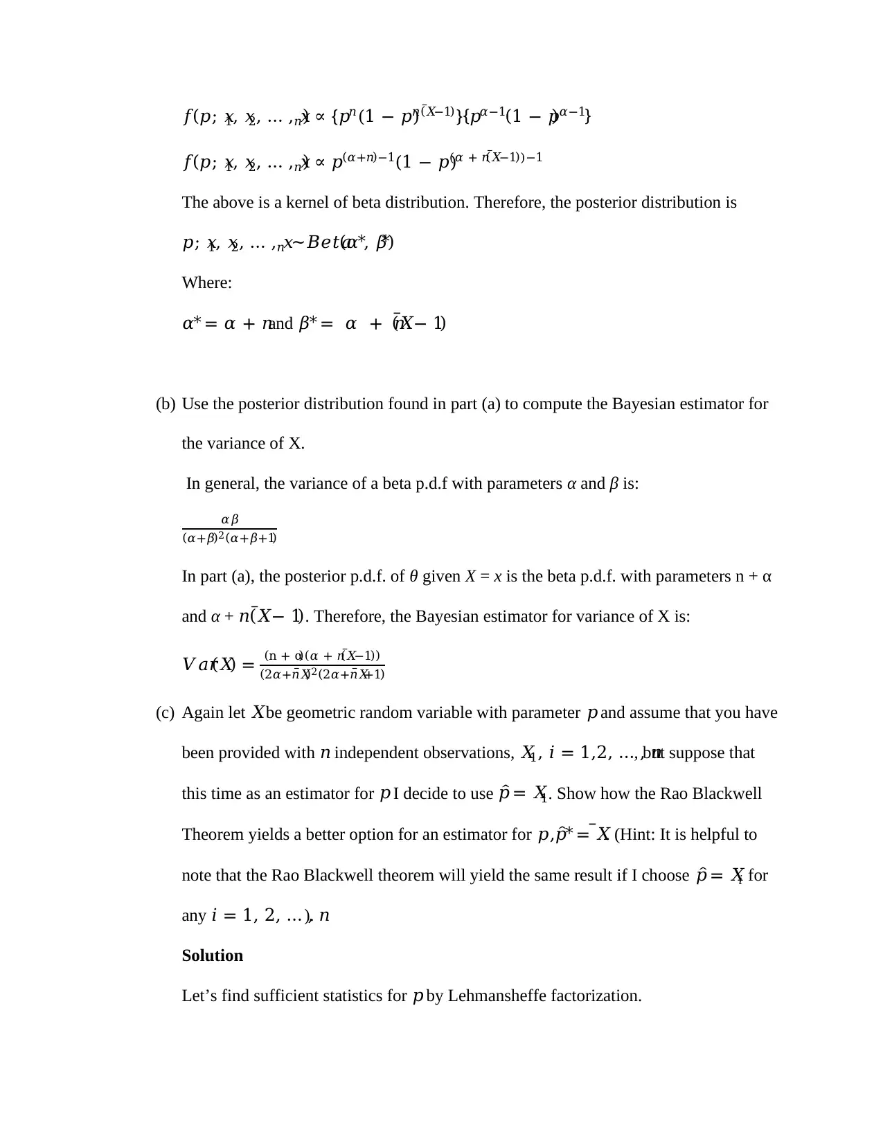
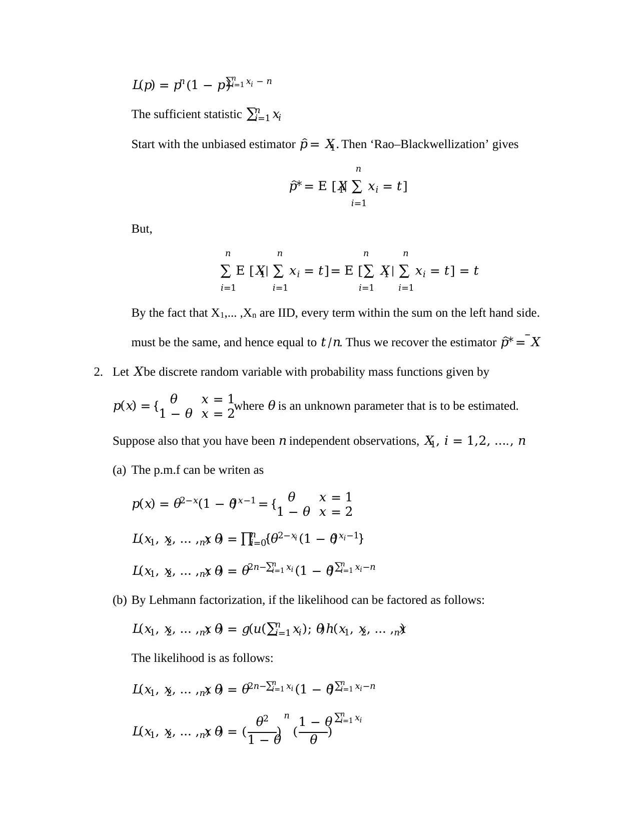
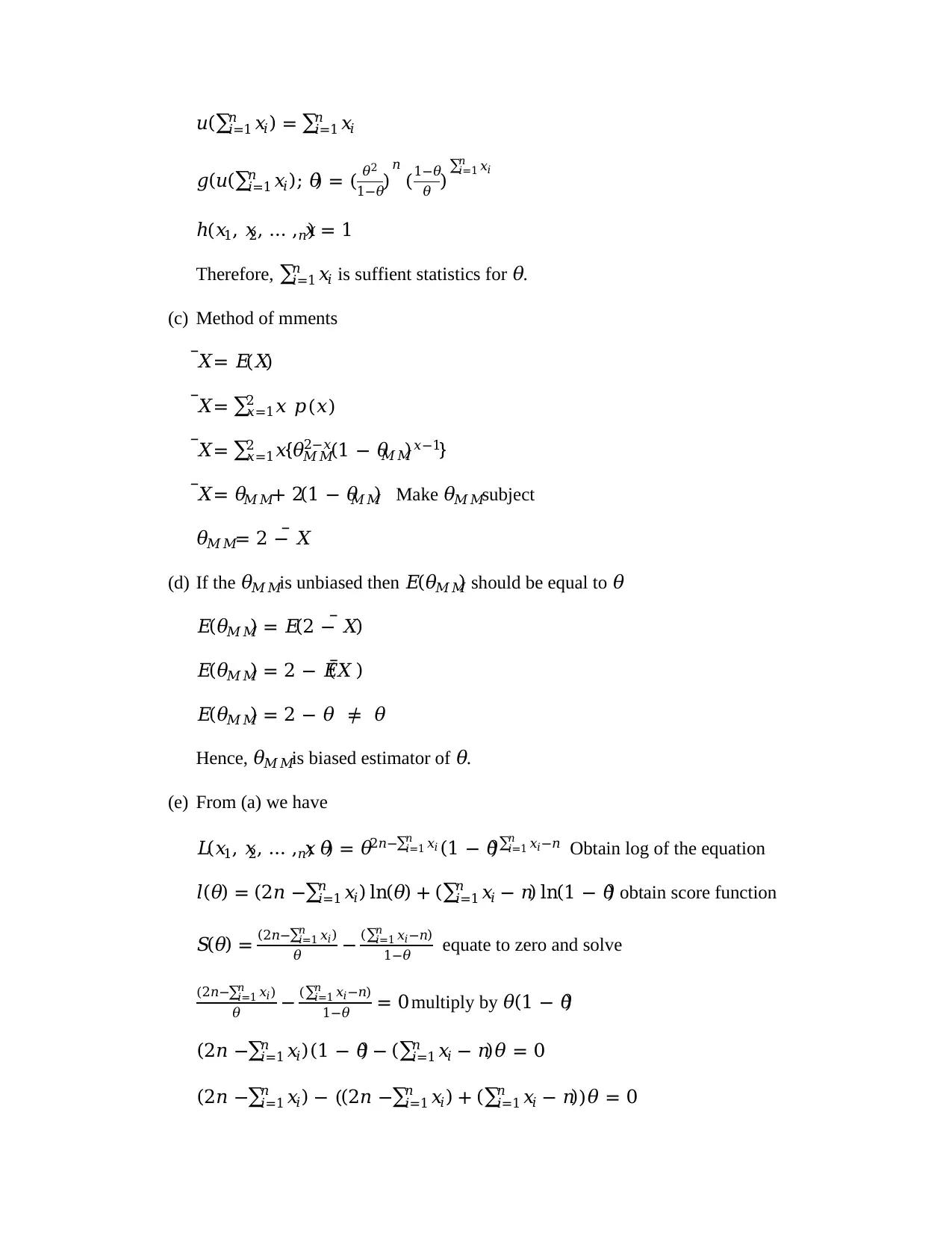
This homework assignment provides detailed solutions to several statistical inference problems. It begins with Bayesian estimation for a geometric distribution, including finding the posterior distribution and Bayesian estimator for variance. The solution demonstrates the application of the Rao-Blackwell theorem to find a better estimator for the parameter p. The assignment then moves on to a discrete random variable problem, covering the likelihood function, sufficient statistics, method of moments, and maximum likelihood estimation. It explores the bias of estimators and derives Bayesian estimators. Finally, the assignment addresses confidence intervals, hypothesis testing, and ANOVA analysis using data from a statistical experiment, including model estimation and interpretation of results, and a discussion of the Cramer-Rao lower bound.

1. Posterior
(a) Let X be a geometric random variable with parameter 𝑝. Assume you have been
provided with 𝑛 independent observations, 𝑋𝑖, 𝑖 = 1, 2, … , 𝑛. Find the posterior
distribution for the Bayesian estimator for 𝑝, 𝑝𝐵 if you assume a prior distribution for
𝑝 that is uniform on the interval [0, 1]. (Hint: The Beta distribution may be of some
help to you in this endeavor).
Solution
The geometric distribution is given by the p.m.f
Pr(𝑋 = 𝑥; 𝑝) = 𝑝(1 − 𝑝)𝑥−1 , 𝑥 = 1, 2, … 𝑛
Uniform distribution is a special form of beta distribution where the scale and the
shape parameter are equal.
Then, 𝑢𝑛𝑖𝑓𝑜𝑟𝑚(0, 1) ≈ 𝑏𝑒𝑡𝑎(𝛼, 𝛽)where 𝛽 = 𝛼
Therefore, the prior distribution is
𝑓(𝑝; 𝛼, 𝛽) = Γ(2𝛼)
(Γ(𝛼))2 𝑝𝛼−1(1 − 𝑝)𝛼−1 for 𝛼 = 𝛽
By definition posterior distribution is given by the fomula:
𝑓(𝑝; 𝑥1, 𝑥2, … , 𝑥𝑛) = 𝐿(𝑝)𝑓(𝑝; 𝛼, 𝛽)
Where:
𝐿(𝑝) is thelikelihood of the geometric distribution
𝐿(𝑝) = ∏ {𝑝(1 − 𝑝)𝑥𝑖−1}𝑛
𝑖=1
𝐿(𝑝) = 𝑝𝑛(1 − 𝑝)∑ 𝑥𝑖
𝑛
𝑖=1 − 𝑛 but we know that ∑ 𝑥𝑖
𝑛
𝑖=1 = 𝑛𝑋̅
𝐿(𝑝) = 𝑝𝑛(1 − 𝑝)𝑛(𝑋̅−1)
Then,

𝑓(𝑝; 𝑥1, 𝑥2, … , 𝑥𝑛) ∝ {𝑝𝑛(1 − 𝑝)𝑛(𝑋̅−1)}{𝑝𝛼−1(1 − 𝑝)𝛼−1}
𝑓(𝑝; 𝑥1, 𝑥2, … , 𝑥𝑛) ∝ 𝑝(𝛼+𝑛)−1(1 − 𝑝)(𝛼 + 𝑛(𝑋̅−1))−1
The above is a kernel of beta distribution. Therefore, the posterior distribution is
𝑝; 𝑥1, 𝑥2, … , 𝑥𝑛 ~𝐵𝑒𝑡𝑎(𝛼∗
, 𝛽∗)
Where:
𝛼∗ = 𝛼 + 𝑛and 𝛽∗ = 𝛼 + 𝑛(𝑋̅− 1)
(b) Use the posterior distribution found in part (a) to compute the Bayesian estimator for
the variance of X.
In general, the variance of a beta p.d.f with parameters α and β is:
𝛼𝛽
(𝛼+𝛽)2(𝛼+𝛽+1)
In part (a), the posterior p.d.f. of θ given X = x is the beta p.d.f. with parameters n + α
and α + 𝑛(𝑋̅− 1). Therefore, the Bayesian estimator for variance of X is:
𝑉𝑎𝑟(𝑋) = (n + α)(𝛼 + 𝑛(𝑋̅−1))
(2𝛼+𝑛𝑋̅)2(2𝛼+𝑛𝑋̅+1)
(c) Again let 𝑋be geometric random variable with parameter 𝑝 and assume that you have
been provided with 𝑛 independent observations, 𝑋1, 𝑖 = 1,2, … , 𝑛, but suppose that
this time as an estimator for 𝑝 I decide to use 𝑝̂ = 𝑋1. Show how the Rao Blackwell
Theorem yields a better option for an estimator for 𝑝,𝑝̂∗ = 𝑋̅. (Hint: It is helpful to
note that the Rao Blackwell theorem will yield the same result if I choose 𝑝̂ = 𝑋𝑖 for
any 𝑖 = 1, 2, … , 𝑛).
Solution
Let’s find sufficient statistics for 𝑝 by Lehmansheffe factorization.

𝐿(𝑝) = 𝑝𝑛(1 − 𝑝)∑ 𝑥𝑖
𝑛
𝑖=1 − 𝑛
The sufficient statistic ∑ 𝑥𝑖
𝑛
𝑖=1
Start with the unbiased estimator 𝑝̂ = 𝑋1. Then ‘Rao–Blackwellization’ gives
𝑝̂∗ = E [𝑋1| ∑ 𝑥𝑖
𝑛
𝑖=1
= 𝑡]
But,
∑ E [𝑋1| ∑ 𝑥𝑖
𝑛
𝑖=1
= 𝑡]
𝑛
𝑖=1
= E [∑ 𝑋1
𝑛
𝑖=1
| ∑ 𝑥𝑖
𝑛
𝑖=1
= 𝑡] = 𝑡
By the fact that X1,... ,Xn are IID, every term within the sum on the left hand side.
must be the same, and hence equal to 𝑡/𝑛. Thus we recover the estimator 𝑝̂∗ = 𝑋̅
2. Let 𝑋be discrete random variable with probability mass functions given by
𝑝(𝑥) = { 𝜃 𝑥 = 1
1 − 𝜃 𝑥 = 2where 𝜃 is an unknown parameter that is to be estimated.
Suppose also that you have been 𝑛 independent observations, 𝑋1, 𝑖 = 1,2, … , 𝑛.
(a) The p.m.f can be writen as
𝑝(𝑥) = 𝜃2−𝑥(1 − 𝜃)𝑥−1 = { 𝜃 𝑥 = 1
1 − 𝜃 𝑥 = 2
.
𝐿(𝑥1, 𝑥2, … , 𝑥𝑛; 𝜃) = ∏ {𝜃2−𝑥𝑖 (1 − 𝜃)𝑥𝑖−1}𝑛
𝑖=0
𝐿(𝑥1, 𝑥2, … , 𝑥𝑛; 𝜃) = 𝜃2𝑛−∑ 𝑥𝑖
𝑛
𝑖=1 (1 − 𝜃)∑ 𝑥𝑖
𝑛
𝑖=1 −𝑛
(b) By Lehmann factorization, if the likelihood can be factored as follows:
𝐿(𝑥1, 𝑥2, … , 𝑥𝑛; 𝜃) = 𝑔(𝑢(∑ 𝑥𝑖
𝑛
𝑖=1 ); 𝜃)ℎ(𝑥1, 𝑥2, … , 𝑥𝑛)
The likelihood is as follows:
𝐿(𝑥1, 𝑥2, … , 𝑥𝑛; 𝜃) = 𝜃2𝑛−∑ 𝑥𝑖
𝑛
𝑖=1 (1 − 𝜃)∑ 𝑥𝑖
𝑛
𝑖=1 −𝑛
𝐿(𝑥1, 𝑥2, … , 𝑥𝑛; 𝜃) = ( 𝜃2
1 − 𝜃
)
𝑛
(1 − 𝜃
𝜃 )
∑ 𝑥𝑖
𝑛
𝑖=1

𝑢(∑ 𝑥𝑖
𝑛
𝑖=1 ) = ∑ 𝑥𝑖
𝑛
𝑖=1
𝑔(𝑢(∑ 𝑥𝑖
𝑛
𝑖=1 ); 𝜃) = ( 𝜃2
1−𝜃)𝑛
(1−𝜃
𝜃 )∑ 𝑥𝑖
𝑛
𝑖=1
ℎ(𝑥1, 𝑥2, … , 𝑥𝑛) = 1
Therefore, ∑ 𝑥𝑖
𝑛
𝑖=1 is suffient statistics for 𝜃.
(c) Method of mments
𝑋̅= 𝐸(𝑋)
𝑋̅= ∑ 𝑥 𝑝(𝑥)2
𝑥=1
𝑋̅= ∑ 𝑥{𝜃𝑀𝑀
2−𝑥(1 − 𝜃𝑀𝑀)𝑥−1}2
𝑥=1
𝑋̅= 𝜃𝑀𝑀+ 2(1 − 𝜃𝑀𝑀) Make 𝜃𝑀𝑀subject
𝜃𝑀𝑀= 2 − 𝑋̅
(d) If the 𝜃𝑀𝑀is unbiased then 𝐸(𝜃𝑀𝑀) should be equal to 𝜃
𝐸(𝜃𝑀𝑀) = 𝐸(2 − 𝑋̅)
𝐸(𝜃𝑀𝑀) = 2 − 𝐸(𝑋̅ )
𝐸(𝜃𝑀𝑀) = 2 − 𝜃 ≠ 𝜃
Hence, 𝜃𝑀𝑀is biased estimator of 𝜃.
(e) From (a) we have
𝐿(𝑥1, 𝑥2, … , 𝑥𝑛; 𝜃) = 𝜃2𝑛−∑ 𝑥𝑖
𝑛
𝑖=1 (1 − 𝜃)∑ 𝑥𝑖
𝑛
𝑖=1 −𝑛 Obtain log of the equation
𝑙(𝜃) = (2𝑛 −∑ 𝑥𝑖
𝑛
𝑖=1 ) ln(𝜃) + (∑ 𝑥𝑖
𝑛
𝑖=1 − 𝑛) ln(1 − 𝜃) obtain score function
𝑆(𝜃) = (2𝑛−∑ 𝑥𝑖
𝑛
𝑖=1 )
𝜃 − (∑ 𝑥𝑖
𝑛
𝑖=1 −𝑛)
1−𝜃 equate to zero and solve
(2𝑛−∑ 𝑥𝑖
𝑛
𝑖=1 )
𝜃 − (∑ 𝑥𝑖
𝑛
𝑖=1 −𝑛)
1−𝜃 = 0 multiply by 𝜃(1 − 𝜃)
(2𝑛 −∑ 𝑥𝑖
𝑛
𝑖=1 )(1 − 𝜃) − (∑ 𝑥𝑖
𝑛
𝑖=1 − 𝑛)𝜃 = 0
(2𝑛 −∑ 𝑥𝑖
𝑛
𝑖=1 ) − ((2𝑛 −∑ 𝑥𝑖
𝑛
𝑖=1 ) + (∑ 𝑥𝑖
𝑛
𝑖=1 − 𝑛))𝜃 = 0

𝜃𝑀𝐿𝐸= (2𝑛−∑ 𝑥𝑖
𝑛
𝑖=1 )
𝑛
𝜃𝑀𝐿𝐸= 2 − 𝑋̅
(f) If the 𝜃𝑀𝐿𝐸is unbiased then 𝐸(𝜃𝑀𝐿𝐸) should be equal to 𝜃
𝐸(𝜃𝑀𝐿𝐸) = 𝐸(2 − 𝑋̅)
𝐸(𝜃𝑀𝐿𝐸) = 2 − 𝜃 ≠ 𝜃
Hence, 𝜃𝑀𝐿𝐸is biased estimator of 𝜃.
(g) Prior 𝑈(0,1) = 𝐵𝑒𝑡𝑎(𝛼, 𝛼)
𝑓(𝜃) ∝ 𝜃𝛼−1(1 − 𝜃)𝛼−1 prior kernel
Th posterior
𝑓(𝜃; 𝑥1, 𝑥2, … , 𝑥𝑛) ∝ 𝐿(𝑥1, 𝑥2, … , 𝑥𝑛; 𝜃)𝑓(𝜃)
𝑓(𝜃; 𝑥1, 𝑥2, … , 𝑥𝑛) ∝ {𝜃2𝑛−∑ 𝑥𝑖
𝑛
𝑖=1 (1 − 𝜃)∑ 𝑥𝑖
𝑛
𝑖=1 −𝑛}𝜃𝛼−1(1 − 𝜃)𝛼−1
𝑓(𝜃; 𝑥1, 𝑥2, … , 𝑥𝑛) ∝ 𝜃2𝑛+ 𝛼−∑ 𝑥𝑖
𝑛
𝑖=1 −1(1 − 𝜃)𝛼+∑ 𝑥𝑖
𝑛
𝑖=1 −𝑛−1
The posterior is a beta distribution with the following parameters
𝛼∗ = 2𝑛 + 𝛼 −∑ 𝑥𝑖
𝑛
𝑖=1 and 𝛽∗ = 𝛼 +∑ 𝑥𝑖
𝑛
𝑖=1 − 𝑛.
In general, the mean of a beta p.d.f with parameters α and β is:
𝛼
𝛼+𝛽
Therefore, the Bayesian estimator for 𝜃 is:
𝜃𝐵 = 2𝑛+ 𝛼−∑ 𝑥𝑖
𝑛
𝑖=1
𝑛+ 2𝛼 = 𝑛(2−𝑋̅)+ 𝛼
𝑛+ 2𝛼
(h) The estimated beta in (e) is 𝜃𝑀𝐿𝐸= 2 − 𝑋̅and 𝜃𝐵 = 𝑛(2−𝑋̅)+ 𝛼
𝑛+ 2𝛼 . But we can express
𝜃𝐵 as follows:
𝜃𝐵 = 𝑛(𝜃𝑀𝐿𝐸) + 𝛼
𝑛+ 2𝛼

From the above equation it is clear that 𝜃𝐵 is the weighted average of 𝜃𝑀𝐿𝐸.
Further, the posterior is a beta distribution thus its mean is similar to its uniform
equivalent.
(i) If the 𝜃𝐵 is unbiased then 𝐸(𝜃𝐵) should be equal to 𝜃
𝐸(𝜃𝐵) = 𝐸 (
𝑛(2−𝑋̅)+ 𝛼
𝑛+ 2𝛼 )
𝐸(𝜃𝐵) = 𝑛(2−𝜃)+ 𝛼
𝑛+ 2𝛼 ≠ 𝜃
Hence, 𝜃𝐵 is biased estimator of 𝜃.
(j) Given 𝑋1 = 1, 𝑋2 = 2 and 𝑋3 = 3 Then 𝑛 = 3. We have
𝑋̅= 1+2+3
3 = 2
𝜃𝑀𝑀= 2 − 2 = 0= 𝜃𝑀𝐿𝐸
Then,
𝜃𝐵 = 𝑛(𝜃𝑀𝐿𝐸) + 𝛼
𝑛+ 2𝛼 = 𝛼
3+2𝛼
3. Solution
(a) The 90% confidence interval is given by the formula:
(𝑦̅1 − 𝑦̅4) ± 𝑡0.05,𝑑𝑓𝑆𝑦1−𝑦4
Where:
𝑦̅1 = 4.062and 𝑦̅4 = 3.920implying 𝑦̅1 − 𝑦̅4 = 4.062 − 3.920 = 0.142
𝑑𝑓 = 2(𝑛 − 1) = 2(10 − 1) = 18
𝑡0.05,𝑑𝑓= 𝑡0.05,18= 1.734
𝑆𝑦1−𝑦4 = √2𝑀𝑆𝐸
𝑛

𝑀𝑆𝐸 =
𝑆1
2+𝑆4
2
2
𝑆1
2 = ∑ (𝑦1−𝑦̅1)210
𝑖=1
9 = 0.0096
9 = 0.00107
𝑆4
2 = ∑ (𝑦4−𝑦̅4)210
𝑖=1
9 = 0.01
9 = 0.0011
𝑀𝑆𝐸 =
0.00107+0.0011
2 = 0.00109
𝑆𝑦1−𝑦4 = √2(0.00109)
10 = 0.047
Then, the confidence interval is 0.142 ±(1.734 𝑥 0.047) = 0.142 ± 0.081.
Therefore, the 90% is 0.061 ≤ 𝜇1 − 𝜇4 ≤ 0.223.
(b) Hypothesis is given as
𝐻0: 𝜇1 = 𝜇4
𝐻𝑎: 𝜇1 ≠ 𝜇4
Significance level 𝛼 = 0.05
Test statistics t-statistic calculated as follows:
𝑡 = 𝑦̅1−𝑦̅4
√𝑆1
2+𝑆4
2
𝑛
Decision Criteria: Reject Null hypothesis if 𝑡 ≥ 𝑡0.05, 18= 1.734.
Analysis:
𝑡 = 0.142
√0.00107+0.0011
10
= 9.64
Since 𝑡 = 9.64is greater than 1.734 we conclude that at 95% level of confidence the two
means are not equal. The estimated p-value = 0.02.
(c) The ANOVA table is below. The results were obtained from excel attached.
ANOVA table

Source of Variation SS df MS F P-value
Between Groups 0.10082 1 0.10082 92.77914 0.000
Within Groups 0.01956 18 0.001087
Total 0.12038 19
The hypothesis is as follows:
𝐻0: 𝜇1 = 𝜇4 = 0
𝐻𝑎: 𝜇1 ≠ 𝜇4
Significance level 𝛼 = 0.05
Test statistics F-statistic calculated obtained from ANOVA table
Decision Criteria: Reject Null hypothesis if P-value is greater than 𝛼 = 0.05
Since 𝐹1, 18= 92.779has a p-value < 0.000 hence reject the null hypothesis and
conclude that the two means are not equal at 95% confidence level.
(d) The estimated model is as follows:
Coefficients
Standard
Error t Stat P-value
Intercept 4.062 0.010424 389.6653
8.57E-
37
xi -0.142 0.014742 -9.63219
1.58E-
08
Clearly 𝛽̂0 = 4.062 = 𝑦̅1 and 𝛽̂1 = −0.142 = 𝑦̅4 − 𝑦̅1.
(e) From table above t-statistics for 𝛽̂1 = 389.6653with corresponding p-value <
0.000. Therefore, the slope coefficient is significant at 95% level of confidence.
The 95% confidence level is given as follows:
𝛽̂1 ± 𝑆𝐸 = −0.142 ± 0.0147
−0.173 ≤ 𝛽1 ≤ −0.111

(f) Given 𝑌̅ = 𝑌̅1+𝑌̅4
2 we have
(𝑌̅4 − 𝑌̅1)2 = 2((𝑌̅1 − 𝑌̅)2 + (𝑌̅4 − 𝑌̅)2)
We use Right hand side to get left hand side of the equation as follows:
2 {(𝑌̅1 − 𝑌̅1+𝑌̅4
2 )2
+ (𝑌̅4 − 𝑌̅1+𝑌̅4
2 )2
}
2{1
4 (𝑌̅4 − 𝑌̅1)2 + 1
4 (𝑌̅4 − 𝑌̅1)2}
2{1
2 (𝑌̅4 − 𝑌̅1)2} = (𝑌̅4 − 𝑌̅1)2
(g) Let’s take the right-hand side and get the left-hand side of the probability given
𝑃( (𝑡𝑛−2)2 > ( | 𝑌̅4−𝑌̅1|
𝑆𝑝√ 1
𝑛+1
𝑛
)
2
) = 𝑃( (𝑡𝑛−2)2 > | (𝑌̅4−𝑌̅1)2|
(𝑆𝑝√ 1
𝑛+1
𝑛)
2)
𝑃
(
(𝑡𝑛−2)2 > |(𝑌̅4 − 𝑌̅1)2|
(𝑆𝑝√1
𝑛 + 1
𝑛)
2
)
= 𝑃
(
(𝑡𝑛−2)2 > 2((𝑌̅1 − 𝑌̅)2 + (𝑌̅4 − 𝑌̅)2)
(𝑆𝑝√1
𝑛 + 1
𝑛)
2
)
Equivalent to 𝑃( (𝑡𝑛−2) > | 𝑌̅4−𝑌̅1|
𝑆𝑝√ 1
𝑛+1
𝑛
)
4. Solution
(a) The exponential distribution whose 𝐸(𝑋) = 𝜃is defined by pdf
𝑓(𝑥; 𝜃) = 1
𝜃 𝑒−𝑥
𝜃, 𝑥 ≥ 0

(a) The Cramer-Rao lower bound is obtained by the formula.
𝐸 [
𝜕
𝜕𝜃 log{𝑓(𝑥; 𝜃)}]2
log{𝑓(𝑥; 𝜃)} = log (
1
𝜃) − 𝑥
𝜃
𝜕
𝜕𝜃 log{𝑓(𝑥; 𝜃)} = −1
𝜃 + 𝑥
𝜃2 = 𝑥−𝜃
𝜃2
( 𝜕
𝜕𝜃 log{𝑓(𝑥; 𝜃)})2
= (𝑥−𝜃)2
𝜃4
𝐸 [
𝜕
𝜕𝜃 log{𝑓(𝑥; 𝜃)}]2
= 𝐸(𝑥−𝜃)2
𝜃4
𝐸(𝑥−𝜃)2
𝜃4 = 𝑉𝑎𝑟(𝑥)
𝜃4
𝐸 [
𝜕
𝜕𝜃 log{𝑓(𝑥; 𝜃)}]2
= 1
𝜃2
The variance of the lower bound is found as follows:
𝑉𝑎𝑟(𝑔(𝑥)) ≥ 1
𝐸[𝜕
𝜕𝜃 log{𝑓(𝑥;𝜃)}]2
𝑉𝑎𝑟(𝑔(𝑥)) ≥ 𝜃2 Hence, the bound is obtained.
(b) If the 𝑛
𝑛+1 𝑋̅𝑛
2 is unbiased estimator of 𝜃2then 𝐸 ( 𝑛
𝑛+1 𝑋̅𝑛
2 ) should be equal to 𝜃2
𝐸 ( 𝑛
𝑛+1 𝑋̅𝑛
2 ) = 𝑛
𝑛+1 (𝐸(𝑋̅𝑛))2
But, 𝐸(𝑋̅𝑛) = 𝜃
𝑛. Then we have
𝐸 ( 𝑛
𝑛+1 𝑋̅𝑛
2 ) = 𝑛
𝑛+1 (𝜃
𝑛)2
𝐸 ( 𝑛
𝑛+1 𝑋̅𝑛
2 ) = 𝜃2
𝑛(𝑛+1)
𝐸 ( 𝑛
𝑛+1 𝑋̅𝑛
2 ) = 𝜃2
𝑛(𝑛+1) ≠ 𝜃2
Hence, 𝑛
𝑛+1 𝑋̅𝑛
2 is biased estimator of 𝜃2.

(c) The Cramer-Rao lower bound is obtained as described in part (a)