Bayesian Statistics Homework: Posterior Distributions and R Analysis

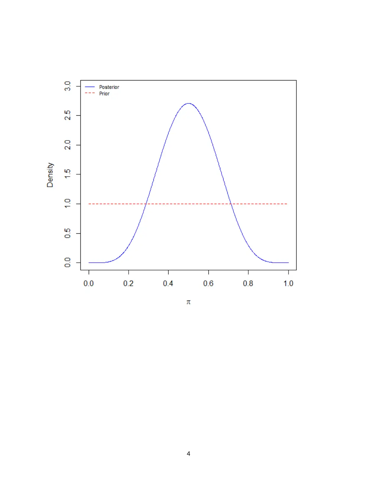
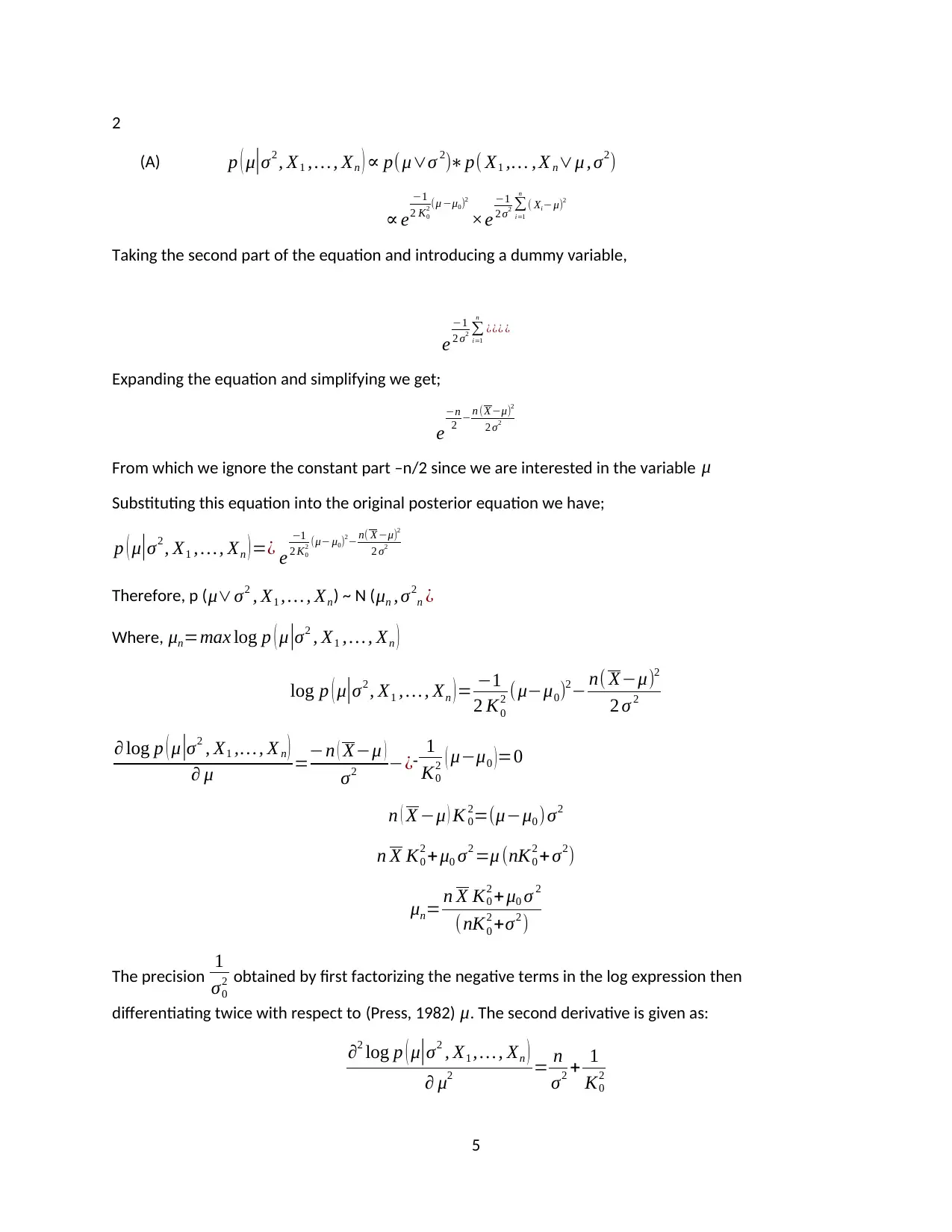
This document provides a comprehensive solution to a Bayesian statistics homework assignment. The assignment focuses on calculating and analyzing posterior distributions under different prior assumptions. Part 1 addresses a binomial distribution with a uniform prior, calculating the posterior distribution and using R to determine the mean, median, standard deviation, and confidence intervals, with a plot demonstrating the results. Part 2 explores a normal distribution with a semi-conjugate prior, calculating the full conditional posterior distributions for both the mean and the variance. The solution includes detailed mathematical derivations and the R code used for the analysis, offering a complete understanding of the concepts and methods involved in Bayesian statistical inference. The assignment references key statistical concepts and provides a practical application of Bayesian methods.

Name:
Institution:
1

Assignment solutions
1
(A) X1 , … , Xn Bin ( n , θ )
Prior unif ( 0,1 )
Posterior ∝likelihood × prior distribution CITATION Mon92 \l 1033 (Monahan & Boos, 1992)
∝¿
∝Constant×θ∑
i=1
n
X i
(1−θ)n−¿∑
i=1
n
Xi ¿
∝θ∑
i=1
n
X i
( 1−θ )n−¿∑
i=1
n
Xi ¿
∝ Beta (∑
i=1
n
Xi +1 , n−∑
i=1
n
Xi+ 1)
(B) The codes and the results are given as below ( copy-pasted from R-console):
Codes
library(Bolstad)
## assuming x=5 successes in n=10 trials
##unif(0,1)is the same as beta(1,1)
kiwi<-binobp(x=5, n=10, a = 1, b = 1, pi = seq(0, 1, by = 0.001), plot = TRUE)
attributes(kiwi)
ki<-kiwi$mean
ki
kii<-kiwi$sd
kii
kiii<-kiwi$var
kiii
##p1 is parameter 1, p2 is parameter 2 that is and b respectively
p1_plus_p2<-(ki*(1-ki)/kiii)-1
p1_plus_p2
newp1<-ki*p1_plus_p2
newp1
newp2<-p1_plus_p2-newp1
newp2
#median
qbeta(0.5,newp1,newp2)
#95% confidence interval
qbeta(0.025,newp1,newp2)
qbeta(0.975,newp1,newp2)
output
> kii<-kiwi$sd
2

> kii
[1] 0.138675
> kiii<-kiwi$var
> kiii
[1] 0.01923077
> ##p1 is parameter 1, p2 is parameter 2 that is and b respectively
> p1_plus_p2<-(ki*(1-ki)/kiii)-1
> p1_plus_p2
[1] 12
> newp1<-ki*p1_plus_p2
> newp1
[1] 6
> newp2<-p1_plus_p2-newp1
> newp2
[1] 6
> #median
> qbeta(0.5,newp1,newp2)
[1] 0.5
> #95% confidence interval
> qbeta(0.025,newp1,newp2)
[1] 0.2337936
> qbeta(0.975,newp1,newp2)
[1] 0.7662064
Plot
3

4

2
(A) p ( μ|σ2 , X1 , … , Xn ) ∝ p(μ∨σ 2)∗p( X1 ,… , X n∨μ , σ2)
∝ e
−1
2 K0
2 (μ −μ0)2
×e
−1
2 σ2 ∑
i=1
n
( Xi− μ)2
Taking the second part of the equation and introducing a dummy variable,
e
−1
2 σ2 ∑
i=1
n
¿¿¿ ¿
Expanding the equation and simplifying we get;
e
−n
2 − n (X −μ)2
2 σ2
From which we ignore the constant part –n/2 since we are interested in the variable μ
Substituting this equation into the original posterior equation we have;
p ( μ|σ2 , X1 , … , Xn )=¿ e
−1
2 K0
2 (μ− μ0)2− n( X −μ)2
2 σ2
Therefore, p ( μ∨σ2 , X1 , … , Xn) ~ N ( μn , σ2
n ¿
Where, μn=max log p ( μ |σ2 , X1 , … , Xn )
log p ( μ|σ2 , X1 , … , Xn ) = −1
2 K0
2 ( μ−μ0)2− n( X−μ)2
2 σ 2
∂ log p ( μ|σ2 , X1 ,… , X n )
∂ μ =−n ( X−μ )
σ2 −¿- 1
K0
2 ( μ−μ0 )=0
n ( X −μ ) K 0
2=(μ−μ0 ) σ2
n X K0
2 + μ0 σ2 =μ (nK0
2 + σ2)
μn= n X K0
2 + μ0 σ 2
(nK0
2 +σ2 )
The precision 1
σ0
2 obtained by first factorizing the negative terms in the log expression then
differentiating twice with respect to (Press, 1982) μ. The second derivative is given as:
∂2 log p ( μ|σ2 , X1 , … , Xn )
∂ μ2 = n
σ2 + 1
K0
2
5

Therefore, ( μ|σ2 , X1 , … , Xn ) N ( n X K0
2 +μ0 σ 2
( nK0
2 +σ2
) , ( n
σ2 + 1
K0
2 )−1
)
(B) p ( σ 2
|μ , X1 , … , Xn ) ∝ p ( σ 2
|μ )∗p ( X1 , … , Xn|μ , σ2 )
p (σ 2
|μ , X1 , … , Xn ) ∝(σ−2)
n
2 e−σ−2
∑
i=1
n
(X i−μ)2
2 ×(σ−2)
v0
2 −1
e− v0 σ0
2
2 σ
−2
∝(σ−2)
n
2 + v0
2 −1
e{−σ−2
(v0 σ 0
2+
∑
i=1
n
( X i−μ )2
2 )}
∝ ( σ−2 )
n +v0
2 −1
e{−σ−2 ¿¿
Therefore p (σ 2
|μ , X1 , … , Xn ) inverse gamma[v0 +n , v0 σ 0
2+ n sn
2 ( μ )].
6

References
Monahan, J. F., & Boos, D. D. (1992). Proper likelihoods for Bayesian analysis. Biometrika.
Press, S. J. (1982). Applied Multivariate Analysis: Using Bayesian and Frequentist Methods of Inference.
Krieger Publishing Company, Inc.
7