Quantitative Methods Assignment 3 Solution for BEA140 Students

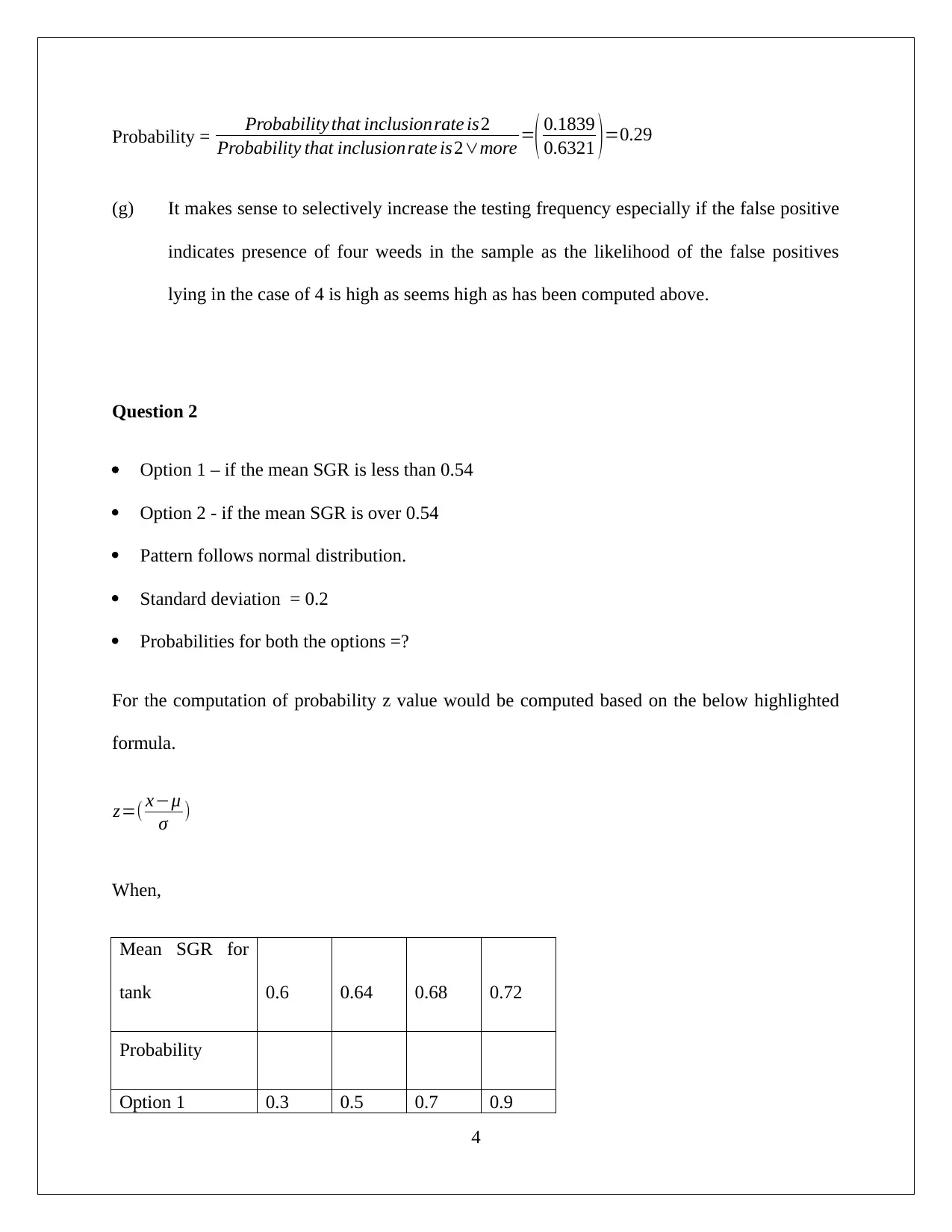
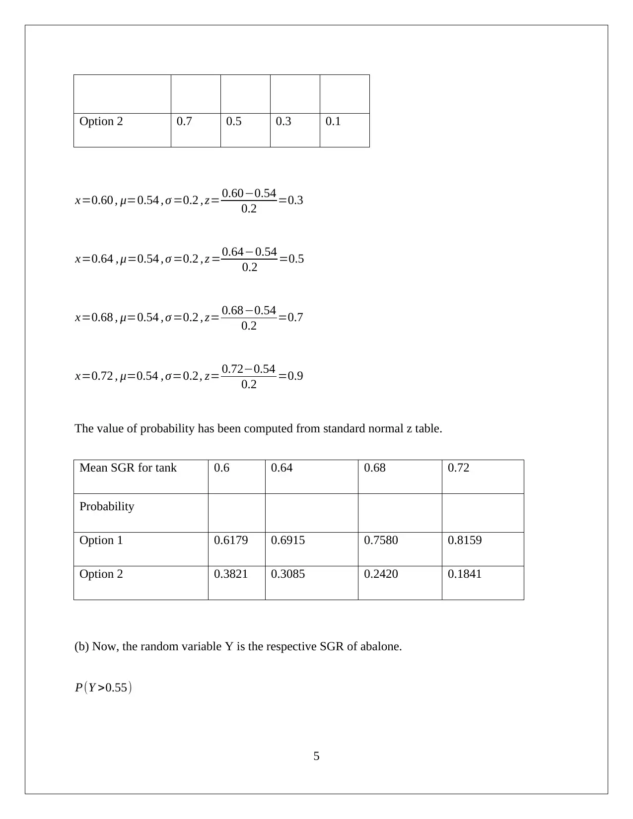
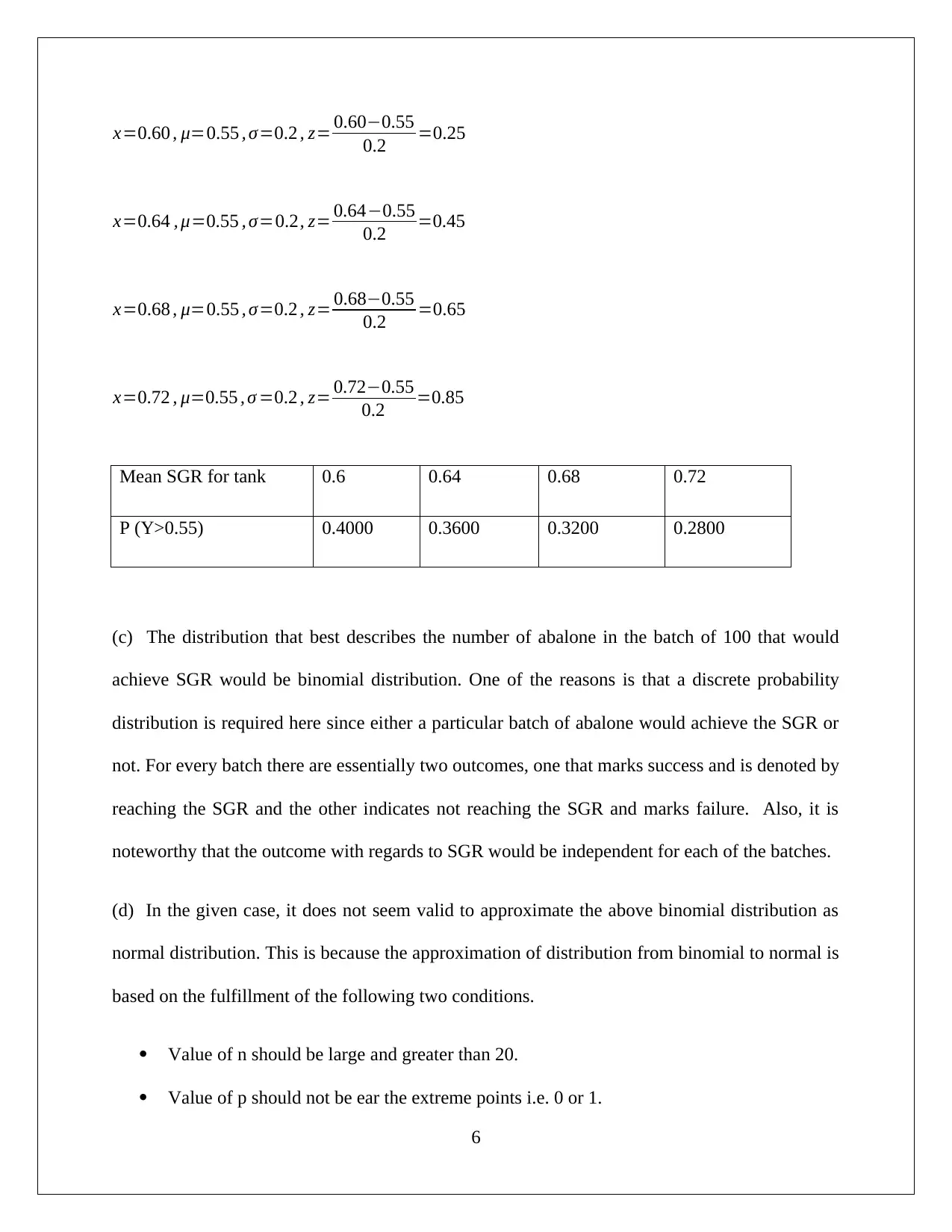
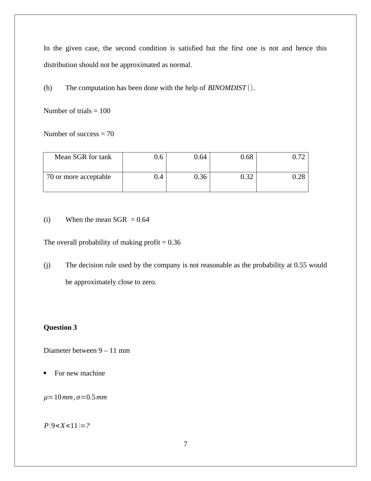
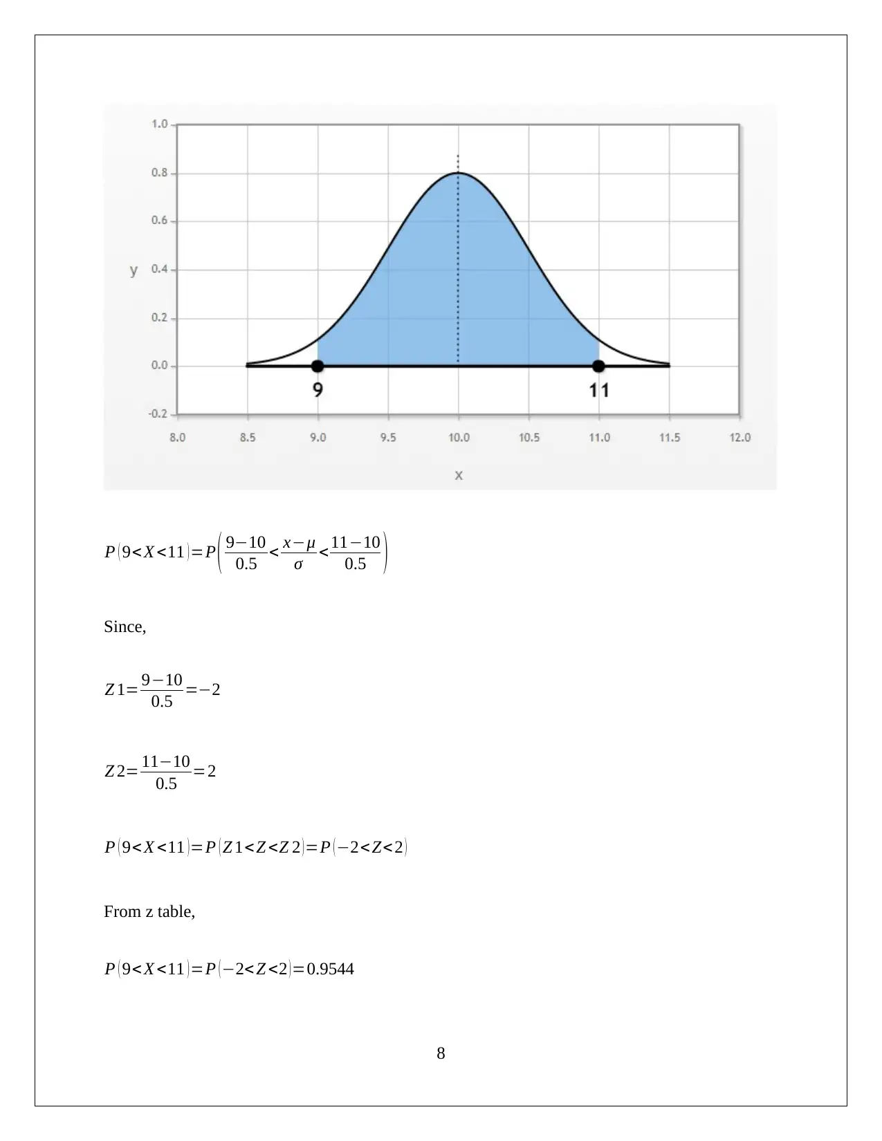
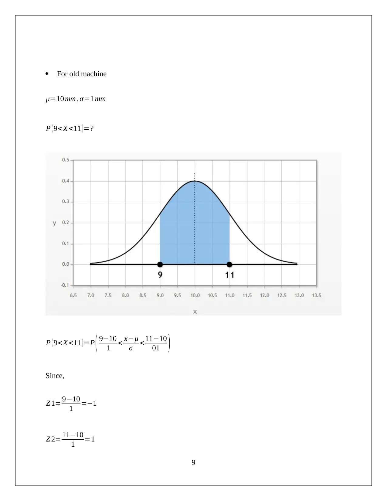
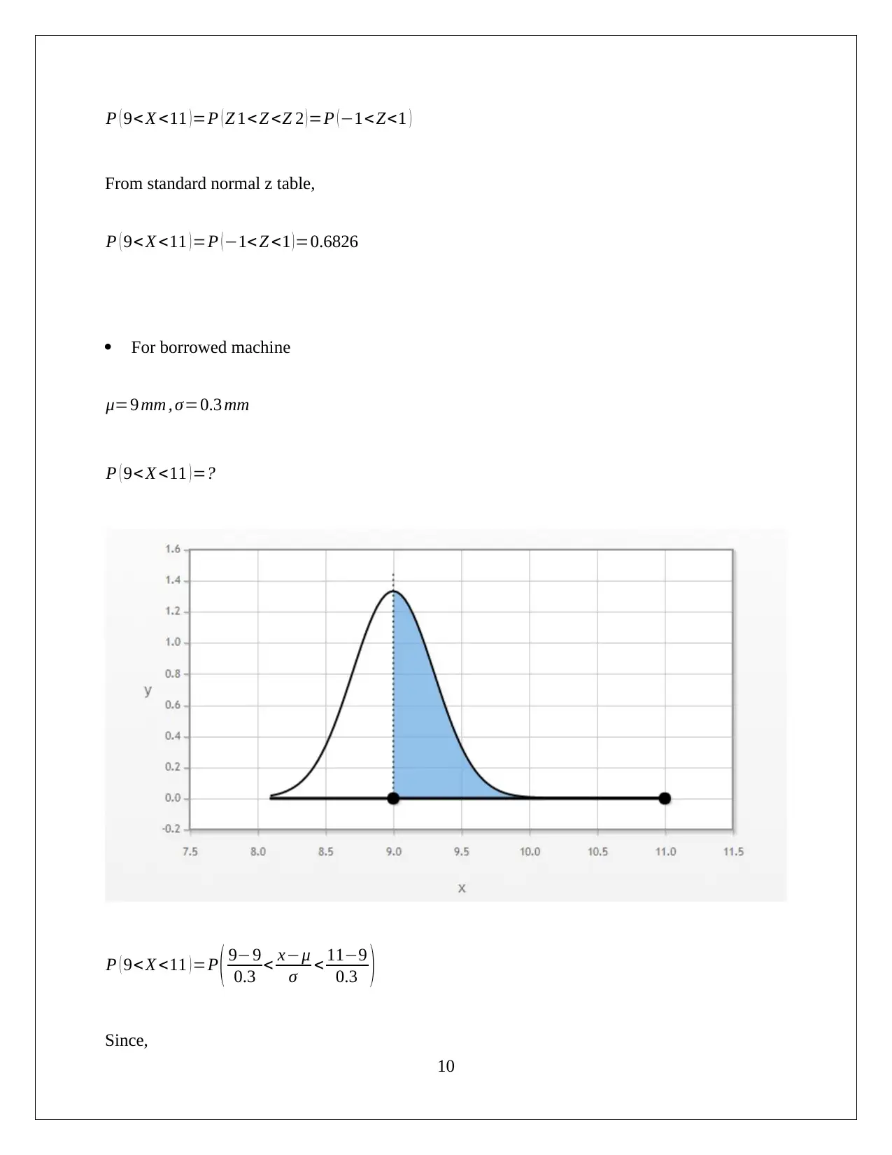
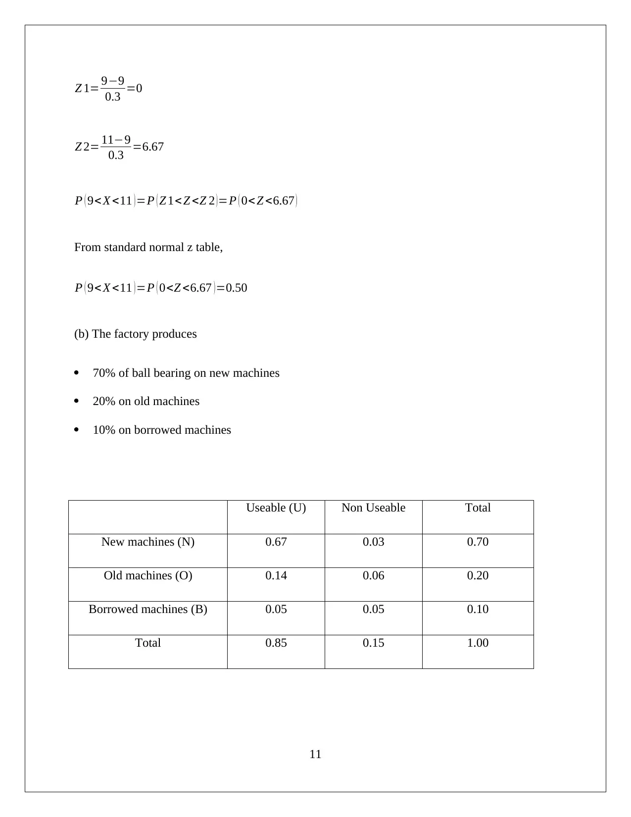
This document presents a complete solution to a Quantitative Methods assignment, likely for a statistics or business analytics course. It covers three main questions. The first question analyzes weed seed distribution using the Poisson distribution, calculating probabilities for different seed counts and determining acceptance criteria based on inclusion rates. The second question delves into the analysis of SGR (Specific Growth Rate) using normal and binomial distributions, calculating probabilities for different SGR values, and evaluating decision rules based on these probabilities. The third question focuses on quality control, analyzing the diameter of ball bearings produced by different machines (new, old, and borrowed) using the normal distribution and calculating conditional probabilities to determine the likelihood of a ball bearing being usable and produced on a new machine. The solution demonstrates the application of various statistical concepts and probability calculations to solve real-world problems, providing a valuable resource for students studying quantitative methods.

Quantitative Methods Assignment 3
BEA140
Student id
[Pick the date]

Question 1
(a) The given number of weeds that would be found in a kg of sample can be approximated
as Poisson distribution. The reasons are as follows.
 Poisson distribution is a discrete probability distribution and the number of weeds would also
be discrete.
 Further, Poisson distribution is based on average incidence of successes that are known
within a region which is known as mean. This value is also known for the given case as 1 per
kg of sample.
(b) Number of seeds found in 1 kg sample = x
Mean value of variable = 1
 Probability of there being 0 seeds observed in 1kg of sample.
Formula for Poisson distribution is shown below:
λ=1 , x=0
P ( X=0 )= e− λ λx
x ! = e−1 10
0! =0.3679
1

 Probability of there being 1 seeds observed in 1kg of sample.
λ=1 , x=1
P ( X=1 ) = e−λ λx
x ! = e−1 11
1 ! =0.3679
 Probability of there being 2 seeds observed in 1kg of sample.
λ=1 , x=2
P ( X=2 )= e−λ λx
x ! = e−1 12
2 ! =0.1839
 Probability of there being 3 seeds observed in 1kg of sample.
λ=1 , x=3
P ( X=3 )= e−λ λx
x ! = e−1 13
3 ! =0.0613
(c) Probability of observing 4 or more seeds in shipment.
λ=1 , x=4
P ( X=4 )=1−{P ( X=0 ) + P ( X =1 ) + P¿
2

¿ 1− ( 0.3679+ 0.3679+0.1839+0.0613 )
¿ 1−0.9810
¿ 0.0190
(d) When λ=2,3,4
Average rate of inclusion in container (seeds per kg)
No of seeds detected in
sample 1 2 3 4
0 0.3679 0.1353 0.0498 0.0183
1 0.3679 0.2707 0.1494 0.0733
2 0.1839 0.2707 0.2240 0.1465
3 0.0613 0.1804 0.2240 0.1954
4 or more 0.0190 0.1429 0.3528 0.5665
(e) Probability of accepting a container when the inclusion rate is 4 seeds per kg ¿ ?
Probability = Probability that inclusionrate is 4
Probability that inclusionrate is 4∨more =( 0.0153
0.0190 )=0.807
(f) If the rate of weed seeds per kg = 2
Probability of redirecting a container with inclusion rate 2 seeds per kg ¿ ?
3

Probability = Probability that inclusionrate is2
Probability that inclusionrate is2∨more =( 0.1839
0.6321 )=0.29
(g) It makes sense to selectively increase the testing frequency especially if the false positive
indicates presence of four weeds in the sample as the likelihood of the false positives
lying in the case of 4 is high as seems high as has been computed above.
Question 2
 Option 1 – if the mean SGR is less than 0.54
 Option 2 - if the mean SGR is over 0.54
 Pattern follows normal distribution.
 Standard deviation = 0.2
 Probabilities for both the options =?
For the computation of probability z value would be computed based on the below highlighted
formula.
z=( x−μ
σ )
When,
Mean SGR for
tank 0.6 0.64 0.68 0.72
Probability
Option 1 0.3 0.5 0.7 0.9
4

Option 2 0.7 0.5 0.3 0.1
x=0.60 , μ=0.54 , σ =0.2 , z= 0.60−0.54
0.2 =0.3
x=0.64 , μ=0.54 , σ =0.2 , z =0.64−0.54
0.2 =0.5
x=0.68 , μ=0.54 , σ =0.2 , z= 0.68−0.54
0.2 =0.7
x=0.72 , μ=0.54 , σ=0.2, z= 0.72−0.54
0.2 =0.9
The value of probability has been computed from standard normal z table.
Mean SGR for tank 0.6 0.64 0.68 0.72
Probability
Option 1 0.6179 0.6915 0.7580 0.8159
Option 2 0.3821 0.3085 0.2420 0.1841
(b) Now, the random variable Y is the respective SGR of abalone.
P(Y >0.55)
5

x=0.60 , μ=0.55 , σ=0.2 , z= 0.60−0.55
0.2 =0.25
x=0.64 , μ=0.55 , σ=0.2, z= 0.64−0.55
0.2 =0.45
x=0.68 , μ=0.55 , σ=0.2 , z= 0.68−0.55
0.2 =0.65
x=0.72 , μ=0.55 , σ =0.2 , z= 0.72−0.55
0.2 =0.85
Mean SGR for tank 0.6 0.64 0.68 0.72
P (Y>0.55) 0.4000 0.3600 0.3200 0.2800
(c) The distribution that best describes the number of abalone in the batch of 100 that would
achieve SGR would be binomial distribution. One of the reasons is that a discrete probability
distribution is required here since either a particular batch of abalone would achieve the SGR or
not. For every batch there are essentially two outcomes, one that marks success and is denoted by
reaching the SGR and the other indicates not reaching the SGR and marks failure. Also, it is
noteworthy that the outcome with regards to SGR would be independent for each of the batches.
(d) In the given case, it does not seem valid to approximate the above binomial distribution as
normal distribution. This is because the approximation of distribution from binomial to normal is
based on the fulfillment of the following two conditions.
 Value of n should be large and greater than 20.
 Value of p should not be ear the extreme points i.e. 0 or 1.
6

In the given case, the second condition is satisfied but the first one is not and hence this
distribution should not be approximated as normal.
(h) The computation has been done with the help of BINOMDIST () .
Number of trials = 100
Number of success = 70
Mean SGR for tank 0.6 0.64 0.68 0.72
70 or more acceptable 0.4 0.36 0.32 0.28
(i) When the mean SGR = 0.64
The overall probability of making profit = 0.36
(j) The decision rule used by the company is not reasonable as the probability at 0.55 would
be approximately close to zero.
Question 3
Diameter between 9 – 11 mm
 For new machine
μ=10 mm , σ=0.5 mm
P ( 9< X <11 )=?
7

P ( 9< X <11 )=P ( 9−10
0.5 < x−μ
σ < 11−10
0.5 )
Since,
Z 1= 9−10
0.5 =−2
Z 2= 11−10
0.5 =2
P ( 9< X <11 ) =P ( Z 1<Z <Z 2 ) =P ( −2<Z<2 )
From z table,
P ( 9< X <11 )=P (−2< Z <2 )=0.9544
8

 For old machine
μ=10 mm , σ=1 mm
P ( 9< X <11 )=?
P ( 9< X <11 )=P ( 9−10
1 < x−μ
σ < 11−10
01 )
Since,
Z 1= 9−10
1 =−1
Z 2= 11−10
1 =1
9

P ( 9< X <11 ) =P ( Z 1<Z <Z 2 ) =P ( −1<Z<1 )
From standard normal z table,
P ( 9< X <11 )=P (−1< Z <1 )=0.6826
 For borrowed machine
μ=9 mm , σ=0.3 mm
P ( 9< X <11 )=?
P ( 9< X <11 )=P ( 9−9
0.3 < x−μ
σ < 11−9
0.3 )
Since,
10

Z 1= 9−9
0.3 =0
Z 2= 11−9
0.3 =6.67
P ( 9< X <11 )=P ( Z 1< Z <Z 2 )=P ( 0< Z <6.67 )
From standard normal z table,
P ( 9< X <11 )=P ( 0<Z <6.67 )=0.50
(b) The factory produces
 70% of ball bearing on new machines
 20% on old machines
 10% on borrowed machines
Useable (U) Non Useable Total
New machines (N) 0.67 0.03 0.70
Old machines (O) 0.14 0.06 0.20
Borrowed machines (B) 0.05 0.05 0.10
Total 0.85 0.15 1.00
11

(c) Conditional probability that a randomly selected ball bearing turns out to be useable and
made on the new machine.
P ( A |B )= P( A ∩ B)
P ( B )
Now,
P (B) sum of probability that is useable = 0.85
P ( A ∩B ) Probability that ball bearing turns out to be useable and new machine = 0.67
P ( A |B )= P ( A ∩ B )
P ( B ) = ( 0.67
0.85 )=0.78
Hence, the requisite conditional probability is 0.78.
12