BEHAVIOURAL ECONOMICS (S1 2019) Assignment 2: Solutions and Analysis

This document presents a comprehensive solution to Assignment 2 in a Behavioral Economics course. The solution covers multiple-choice questions and problem-solving scenarios. Key topics addressed include expected utility maximization, prospect theory, the Ellsberg Paradox, time consistency, Nash Equilibrium, and various discounting models (exponential and quasi-hyperbolic). The assignment analyzes decision-making under risk and uncertainty, exploring concepts such as reference points, loss aversion, and the impact of present bias on choices. The solution includes graphical representations of utility and value functions, along with detailed explanations of how individuals make decisions in different contexts, such as court cases, purchasing decisions, and group assignments. The assignment also examines the implications of different preference structures on strategic interactions. The solutions provided help students to understand and apply behavioral economic principles to real-world situations.

Course on
BEHAVIOURAL ECONOMICS (S1 2019)
Ralph-Christopher Bayer
Assignment 2
Deadline: End of Week 13 (Sunday June 16th, midnight)
Multiple Choice Questions
1. A person that chooses the alternative that has the highest Expected Value, when risk is
involved, violates the assumptions of expected utility maximization.
True. An individual chooses the outcome with the highest expected utility according to
expected utility maximization. So, on the basis of expected value, the assumption of
expected utility maximization is violated
2. An expected utility maximizer with u(x) = log(x) rejects all fair gambles (i.e. those
with an expected value of zero).
False. Because a common utility model suggested by Bernoulli, himself is logarithmic
function of the gamblers total wealth (x) and the concept of diminishing marginal utility
of money is built into it.
3. Prospect Theory can explain the Ellsberg Paradox.
False. The combining behavioral economic theory known as the prospect theory and it
can explain in Allais paradox not Ellsberg paradox.
1

4. Sophisticated Quasi-Hyperbolic Discounters behave time consistently, as they know
that they will have a present bias in future decisions and therefore act to eliminate the
bias.
True. Hyperbolic discounters behave time inconsistent model of delay discounting.
5. The outcome resulting from a Nash Equilibirum is socially efficient, since in a Nash
Equilibrium all players play best responses to each other.
False. Nash Equilibrium is an outcome in which every player is doing the best possible
can be given other player’s choices. So, no player can benefit from unilaterally
changing his choice.
6. Rational preferences should only depend on the person’s own outcomes (such as their
own consumption, wealth, etc.)
True.
7. Jack, who has the utility function u(x,y) = x − γy, where x is his own material payoff,
while y is the material payoff of his neighbour, can be described as envious.
False
8. Somebody who plays the lottery cannot be an expected utility maximizer.
False
2

9. If somebody is taking drugs, then that does not necessarily mean that she/he cannot be
an exponential discounter.
False
10. The Allais Paradox demonstrates that many humans evaluate the same lotteries
differently if they are combined with the same other lottery.
True. The lotteries are evaluated differently because the earlier ones are nested within
others and the new ones are of compound nature.
3

Problems
1. Lucy has current wealth of $100,000. She has just been sent a notice to pay $500 for
speeding. Lucy decides not to pay and to go to court. There she will either get off
(because of insufficient evidence)and pay nothing or will have to pay the fine plus the
court cost which together amount to $1,000. Lucy sees her chances of getting off at
50%.
(a) Suppose Lucy is an expected utility maximizer. Draw a graph with a utility function
that can explain Lucy’s choice. Clearly label the wealth axis. Mark the expected
utility of going to court and the utility of paying the fine.
Part a )
Current wealth of Lucy w=$ 100,000
Now, in scenario 1 Lucy can go to court and decide not to pay anything and get
which has a probability pr (Q)= 50 % or 0.5
In scenario 2 , she will have to pay the fine and the court expenses amounting to a
total of $ 1000. The probability of paying all the expenses, Pr(E)=50% or 0.5 as
well know
, the Expected utility (EV) =Pr (event 1).Gain from event 1+Pr(event 2). Gain from
event 2 + Pr (event 3). Gain from event +Pr (event n). Gain from event n.
In scenario 1 Lucy’s gain= $ 100,000as she pays nothing in scenario 2 her gain = ($
100,000-$ 1000)=$ 99,000
Lucy’s expected utility from scenario 1(getting off)= Pr(G)Gain from getting off
scenario 1.
=0.5 ($ 100,000)
=$ 50,000
= Ev (G)
Lucy’s expected utility from scenario 2 paying a total of $
1000
Pr (E) Gain from scenario 2
=0.5 ($ 99,00)
=$ 49,500=EV(E)
4

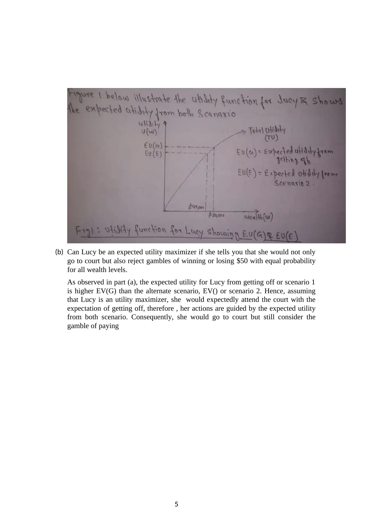
(b) Can Lucy be an expected utility maximizer if she tells you that she would not only
go to court but also reject gambles of winning or losing $50 with equal probability
for all wealth levels.
As observed in part (a), the expected utility for Lucy from getting off or scenario 1
is higher EV(G) than the alternate scenario, EV() or scenario 2. Hence, assuming
that Lucy is an utility maximizer, she would expectedly attend the court with the
expectation of getting off, therefore , her actions are guided by the expected utility
from both scenario. Consequently, she would go to court but still consider the
gamble of paying
5

the fine or getting off as probability of both scenario are equal (50 %) and she can
be better off by getting off.
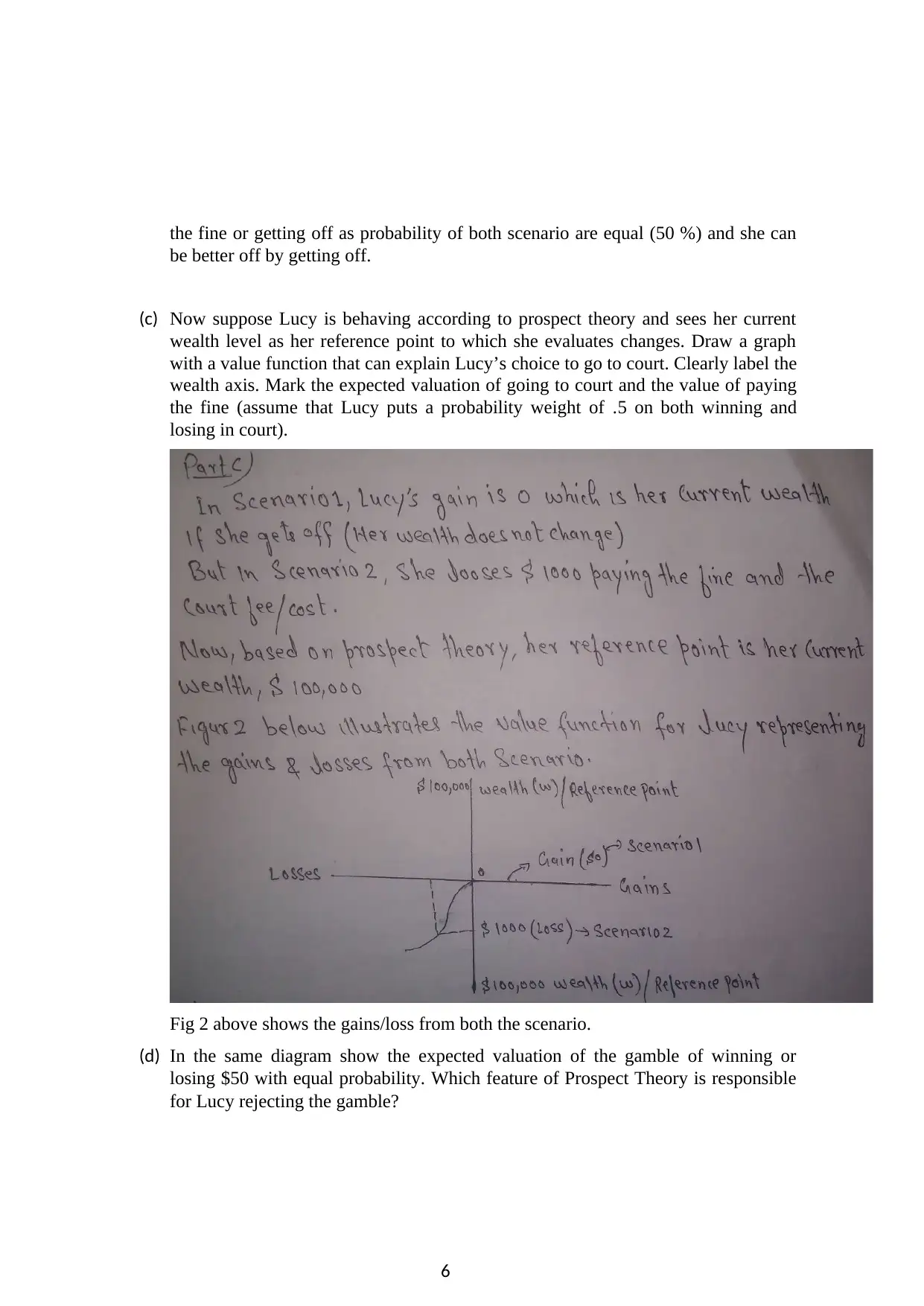
(c) Now suppose Lucy is behaving according to prospect theory and sees her current
wealth level as her reference point to which she evaluates changes. Draw a graph
with a value function that can explain Lucy’s choice to go to court. Clearly label the
wealth axis. Mark the expected valuation of going to court and the value of paying
the fine (assume that Lucy puts a probability weight of .5 on both winning and
losing in court).
Fig 2 above shows the gains/loss from both the scenario.
(d) In the same diagram show the expected valuation of the gamble of winning or
losing $50 with equal probability. Which feature of Prospect Theory is responsible
for Lucy rejecting the gamble?
6

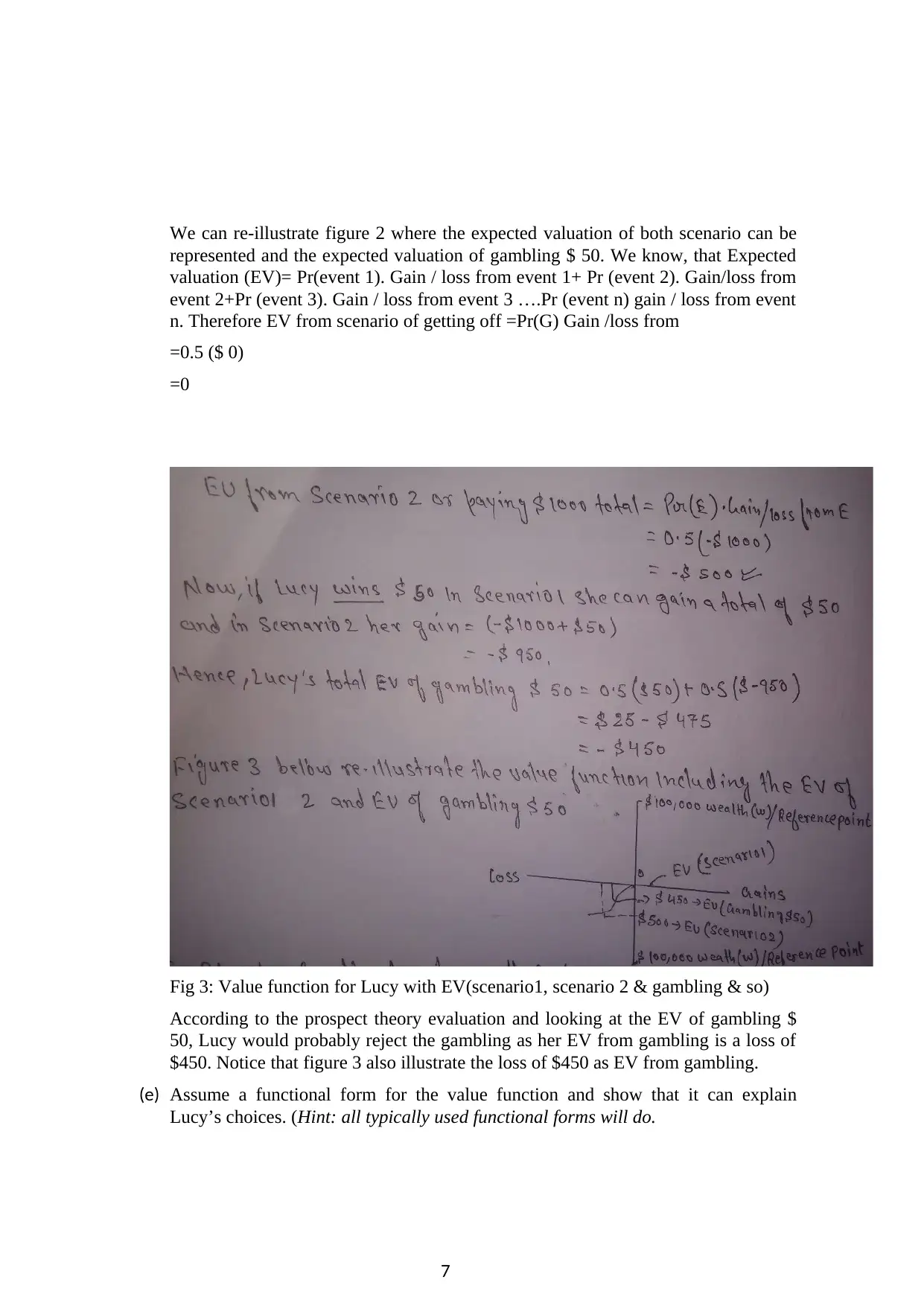
We can re-illustrate figure 2 where the expected valuation of both scenario can be
represented and the expected valuation of gambling $ 50. We know, that Expected
valuation (EV)= Pr(event 1). Gain / loss from event 1+ Pr (event 2). Gain/loss from
event 2+Pr (event 3). Gain / loss from event 3 ….Pr (event n) gain / loss from event
n. Therefore EV from scenario of getting off =Pr(G) Gain /loss from
=0.5 ($ 0)
=0
Fig 3: Value function for Lucy with EV(scenario1, scenario 2 & gambling & so)
According to the prospect theory evaluation and looking at the EV of gambling $
50, Lucy would probably reject the gambling as her EV from gambling is a loss of
$450. Notice that figure 3 also illustrate the loss of $450 as EV from gambling.
(e) Assume a functional form for the value function and show that it can explain
Lucy’s choices. (Hint: all typically used functional forms will do.
7

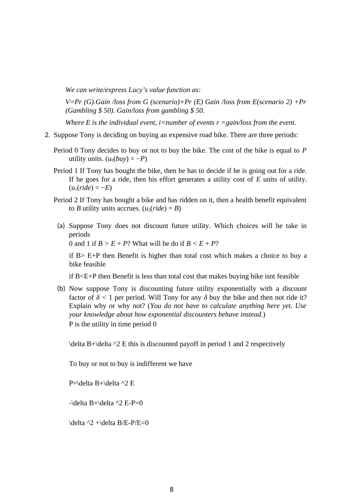
We can write/express Lucy’s value function as:
V=Pr (G).Gain /loss from G (scenario)+Pr (E) Gain /loss from E(scenario 2) +Pr
(Gambling $ 50). Gain/loss from gambling $ 50.
Where E is the individual event, i=number of events r =gain/loss from the event.
2. Suppose Tony is deciding on buying an expensive road bike. There are three periods:
Period 0 Tony decides to buy or not to buy the bike. The cost of the bike is equal to P
utility units. (u0(buy) = −P)
Period 1 If Tony has bought the bike, then he has to decide if he is going out for a ride.
If he goes for a ride, then his effort generates a utility cost of E units of utility.
(u1(ride) = −E)
Period 2 If Tony has bought a bike and has ridden on it, then a health benefit equivalent
to B utility units accrues. (u2(ride) = B)
(a) Suppose Tony does not discount future utility. Which choices will he take in
periods
0 and 1 if B > E + P? What will he do if B < E + P?
if B> E+P then Benefit is higher than total cost which makes a choice to buy a
bike feasible
if B<E+P then Benefit is less than total cost that makes buying bike isnt feasible
(b) Now suppose Tony is discounting future utility exponentially with a discount
factor of δ < 1 per period. Will Tony for any δ buy the bike and then not ride it?
Explain why or why not? (You do not have to calculate anything here yet. Use
your knowledge about how exponential discounters behave instead.)
P is the utility in time period 0
\delta B+\delta ^2 E this is discounted payoff in period 1 and 2 respectively
To buy or not to buy is indifferent we have
P=\delta B+\delta ^2 E
-\delta B+\delta ^2 E-P=0
\delta ^2 +\delta B/E-P/E=0
8

\delta = (-B/E)+sqrt(B^2/E^2+4P/E)/2<1
if \delta>sqrt(B^2/E^2+4P/E) then we can say buying a bike is feasible otherwise
not
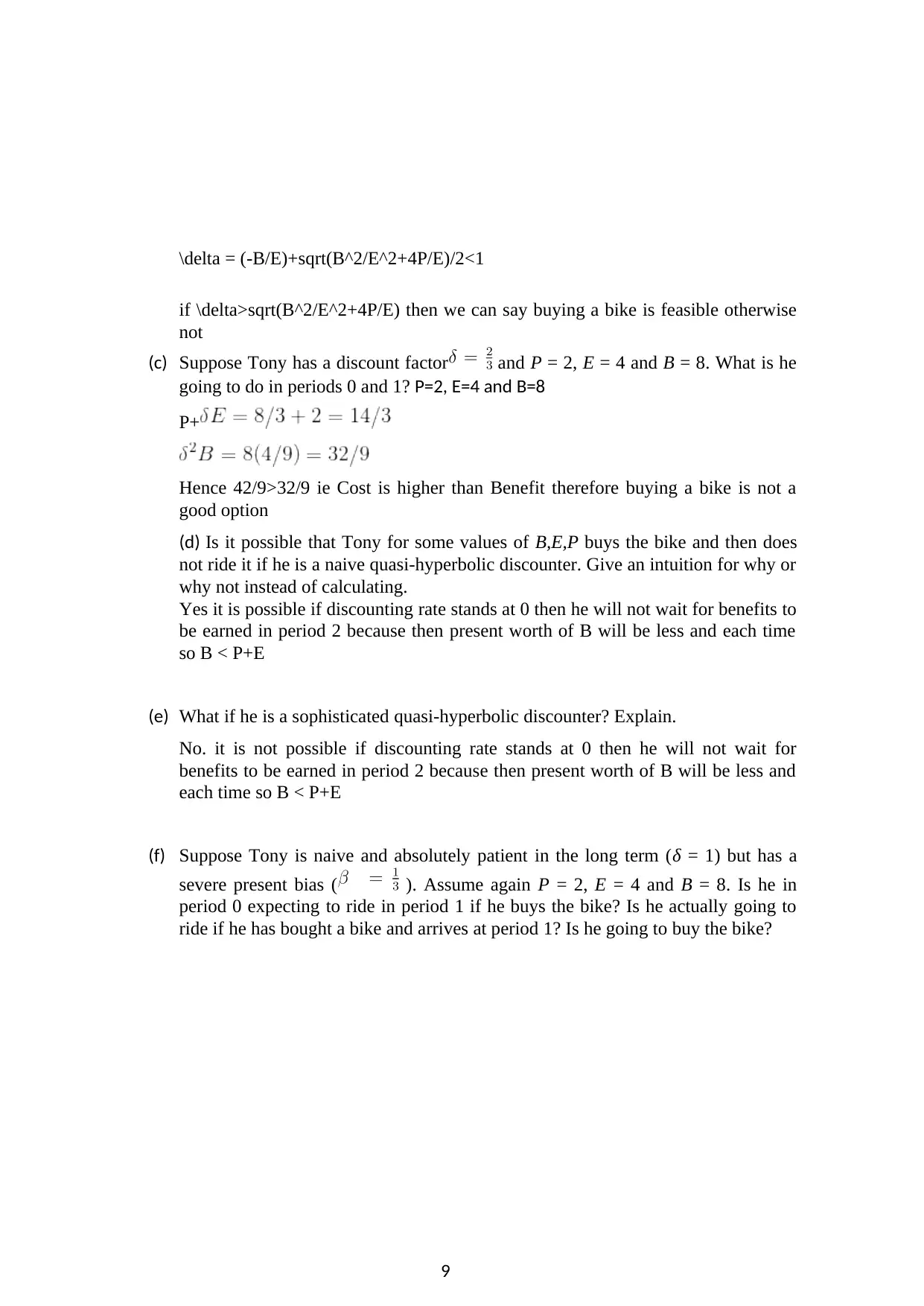
(c) Suppose Tony has a discount factor and P = 2, E = 4 and B = 8. What is he
going to do in periods 0 and 1? P=2, E=4 and B=8
P+
Hence 42/9>32/9 ie Cost is higher than Benefit therefore buying a bike is not a
good option
(d) Is it possible that Tony for some values of B,E,P buys the bike and then does
not ride it if he is a naive quasi-hyperbolic discounter. Give an intuition for why or
why not instead of calculating.
Yes it is possible if discounting rate stands at 0 then he will not wait for benefits to
be earned in period 2 because then present worth of B will be less and each time
so B < P+E
(e) What if he is a sophisticated quasi-hyperbolic discounter? Explain.
No. it is not possible if discounting rate stands at 0 then he will not wait for
benefits to be earned in period 2 because then present worth of B will be less and
each time so B < P+E
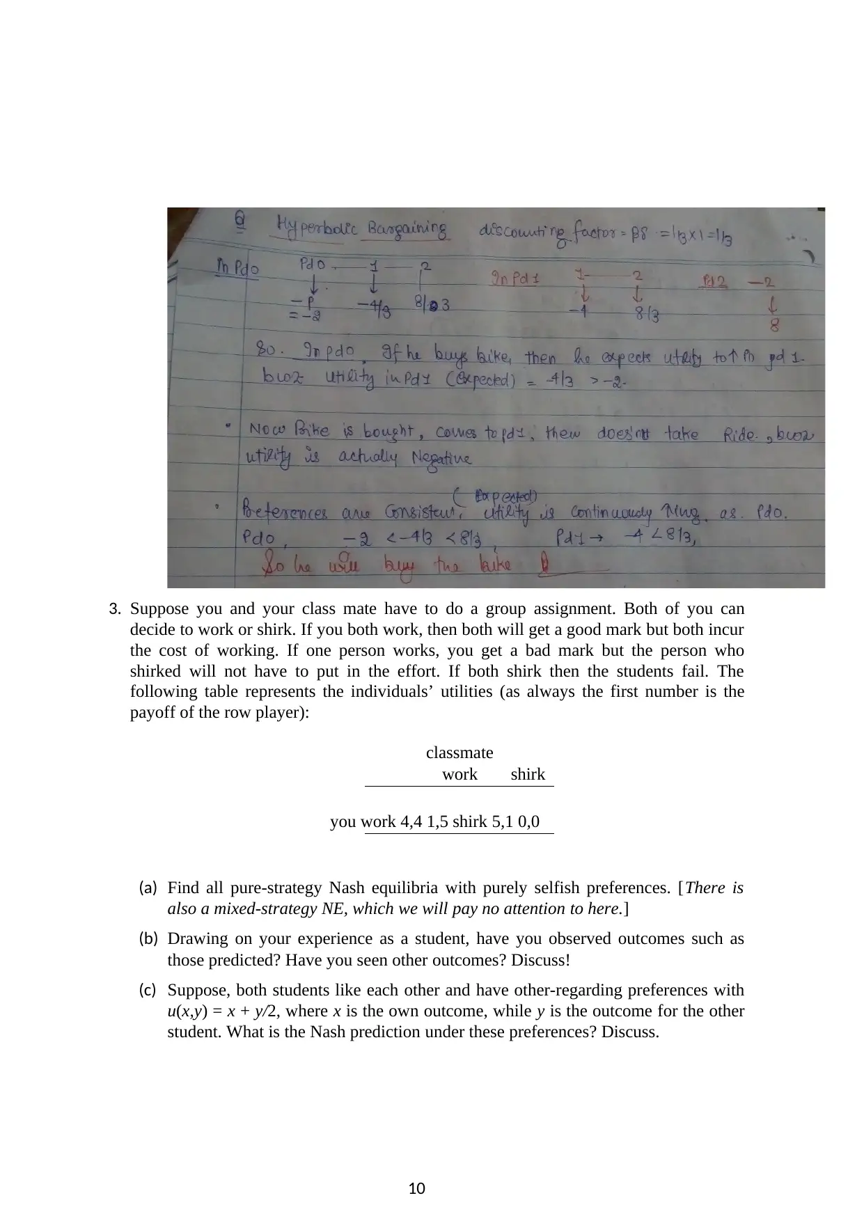
(f) Suppose Tony is naive and absolutely patient in the long term (δ = 1) but has a
severe present bias ( ). Assume again P = 2, E = 4 and B = 8. Is he in
period 0 expecting to ride in period 1 if he buys the bike? Is he actually going to
ride if he has bought a bike and arrives at period 1? Is he going to buy the bike?
9

3. Suppose you and your class mate have to do a group assignment. Both of you can
decide to work or shirk. If you both work, then both will get a good mark but both incur
the cost of working. If one person works, you get a bad mark but the person who
shirked will not have to put in the effort. If both shirk then the students fail. The
following table represents the individuals’ utilities (as always the first number is the
payoff of the row player):
classmate
work shirk
you work 4,4 1,5 shirk 5,1 0,0
(a) Find all pure-strategy Nash equilibria with purely selfish preferences. [There is
also a mixed-strategy NE, which we will pay no attention to here.]
(b) Drawing on your experience as a student, have you observed outcomes such as
those predicted? Have you seen other outcomes? Discuss!
(c) Suppose, both students like each other and have other-regarding preferences with
u(x,y) = x + y/2, where x is the own outcome, while y is the outcome for the other
student. What is the Nash prediction under these preferences? Discuss.
10

(d) Suppose, both students have competitive preferences and care only about how
much better or worse off they are compared to the other student. In other words,
u(x,y) = x − y for both students. What is the Nash prediction now! Discuss.
(e) Suppose both students are inequality averse and lose half a unit of utility for each
unit difference in payoffs. In other words u(x,y) = x−(|x−y|)/2. Find all pure-
strategy Nash equilibria and discuss
All the answers for question a, b, c, d, e,f are provided below
11

12