CIV1900 Coursework: Analysis of Bending Moment Diagrams for Beams

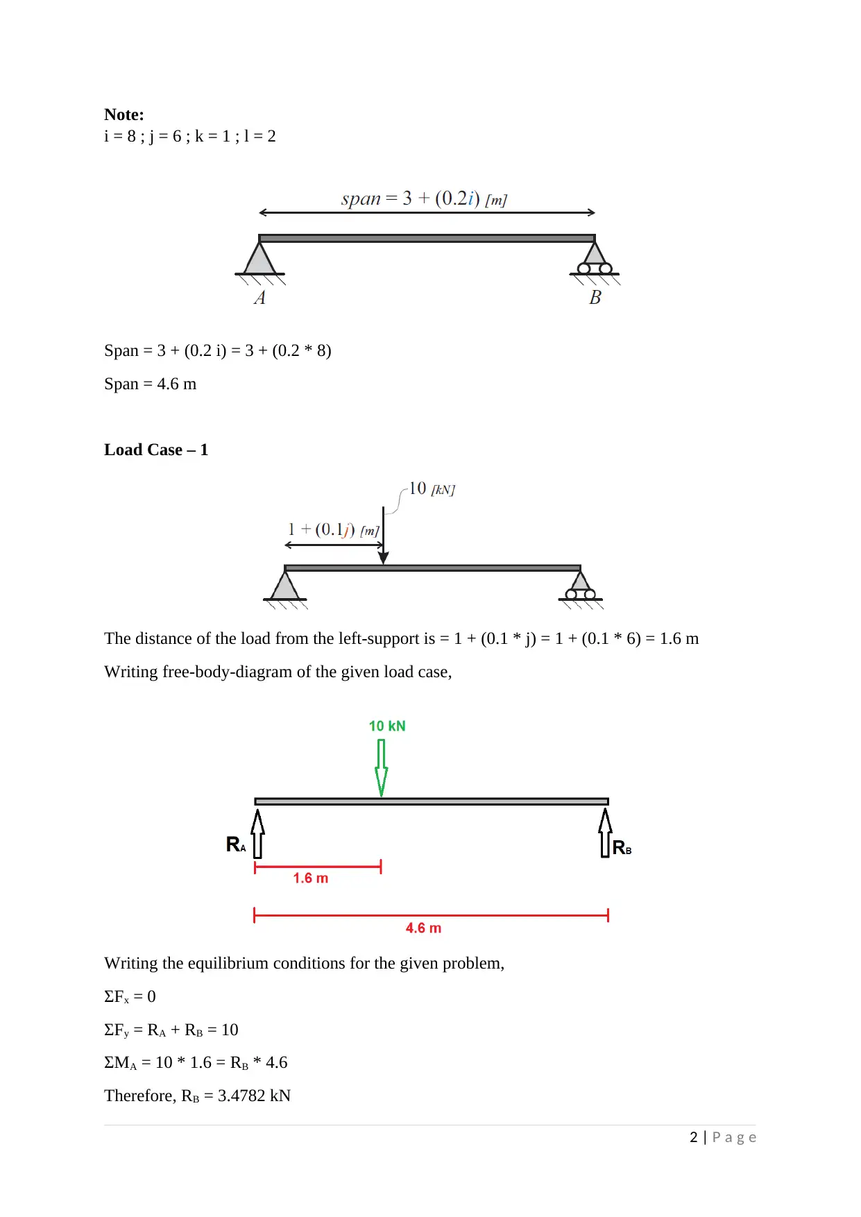
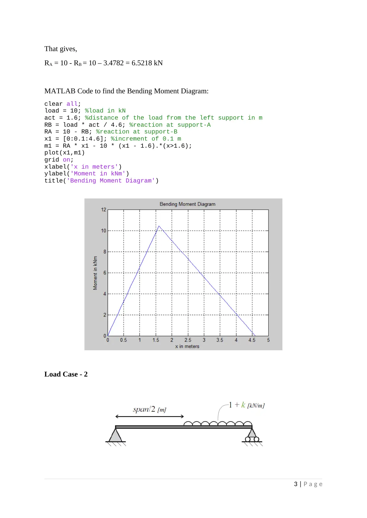
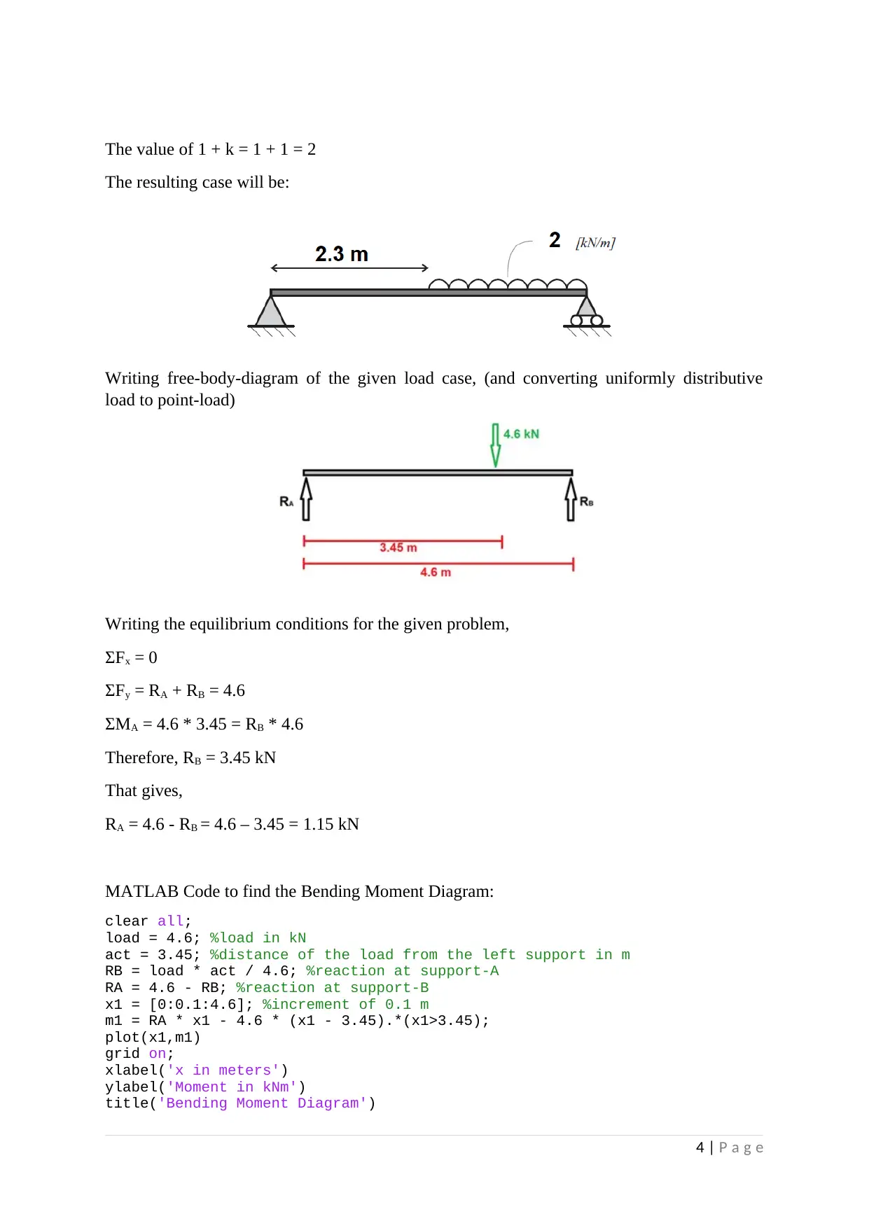
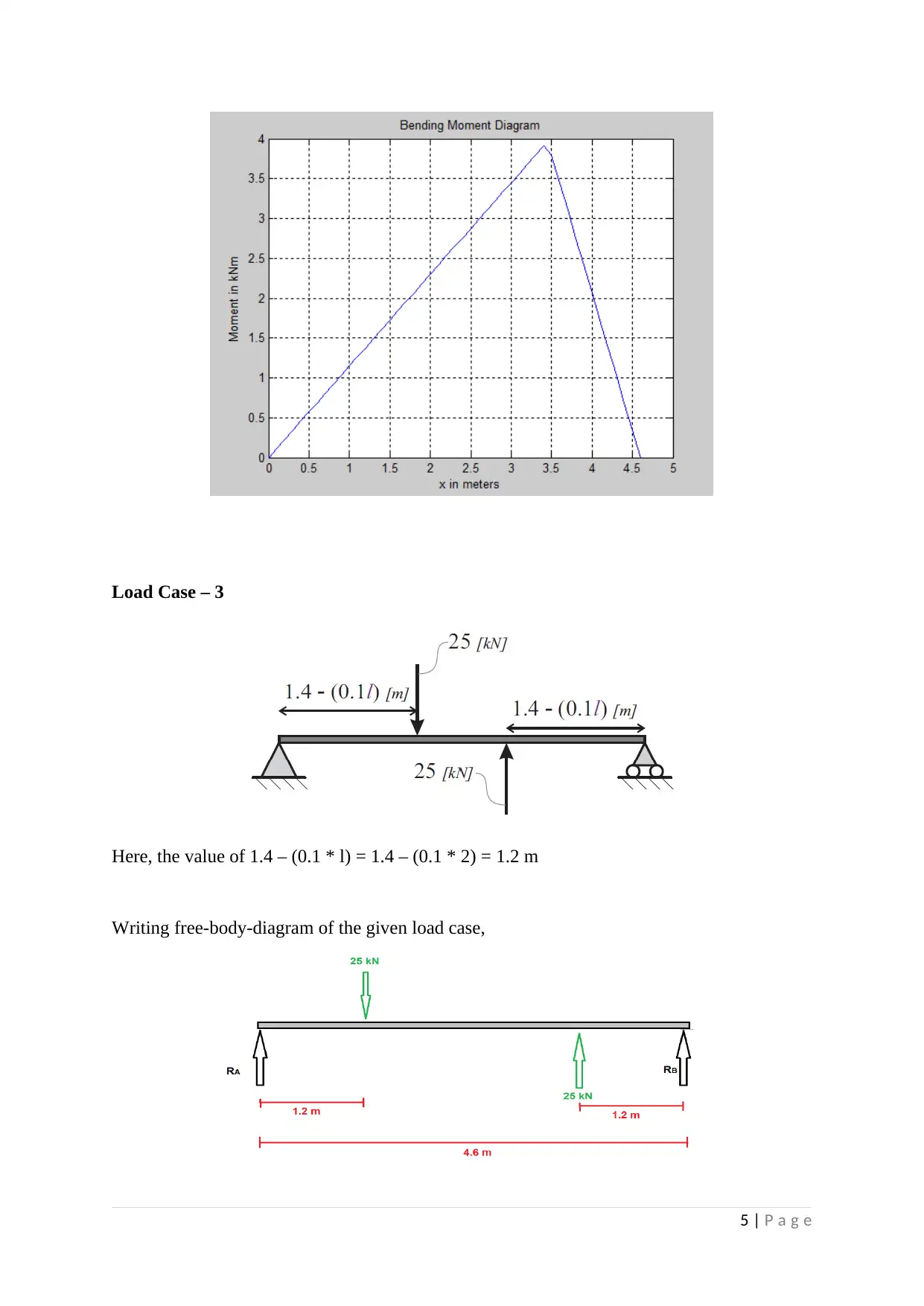
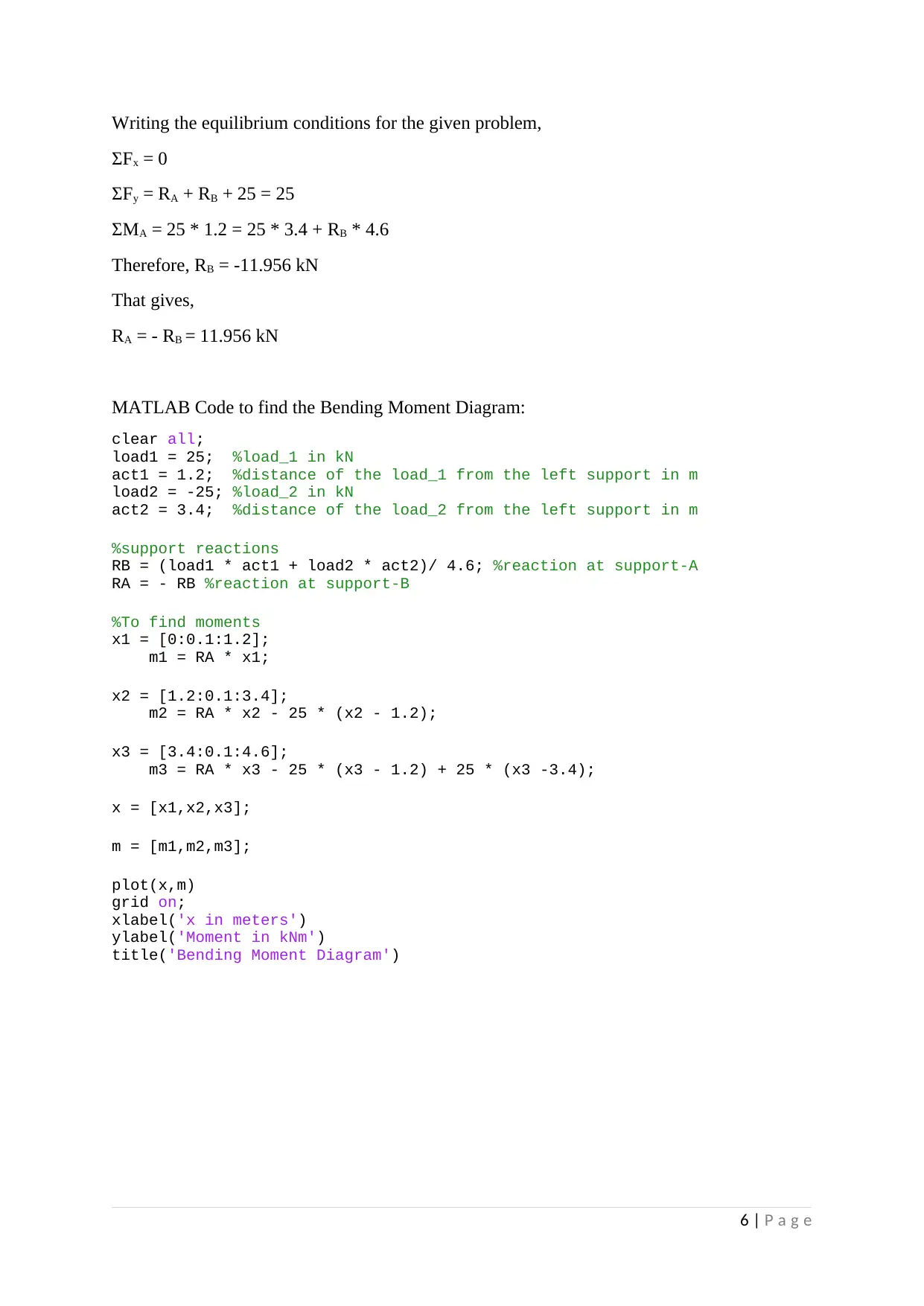
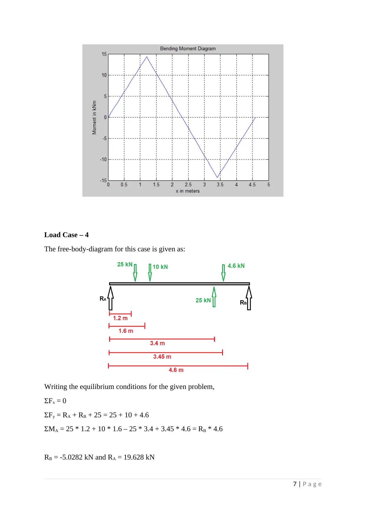
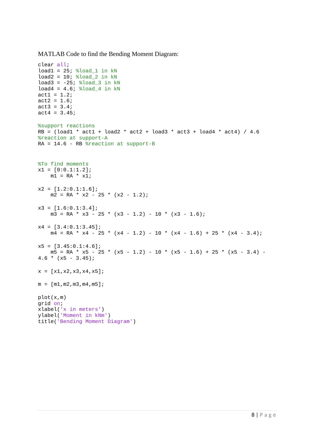
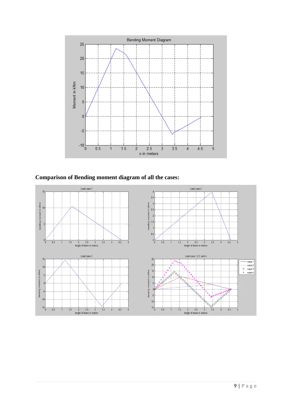
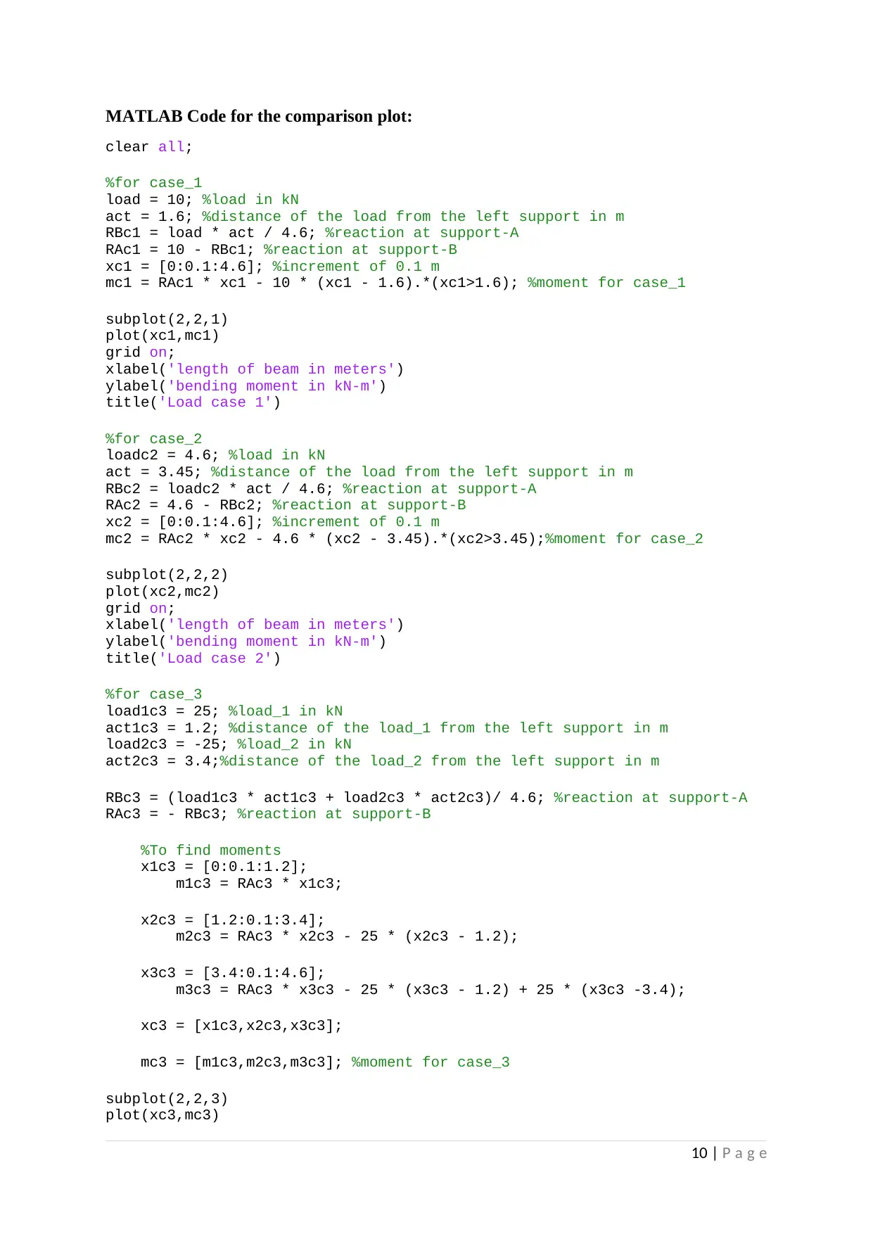
This assignment provides a comprehensive solution to a coursework task involving the calculation and analysis of bending moment diagrams for beams under different loading conditions. The solution includes detailed free-body diagrams, equilibrium conditions, and MATLAB code for generating bending moment diagrams for four distinct load cases. Each load case is thoroughly analyzed, with calculations for support reactions and bending moments at various points along the beam. The MATLAB code is provided for each case, allowing for the visualization of the bending moment distribution. Additionally, the assignment includes solutions to online quiz questions related to the concepts covered, such as calculating reactions, maximum bending moments, and identifying points where the bending moment meets specific criteria. A comparative analysis of the bending moment diagrams for all four cases is also presented, along with MATLAB code for generating the comparison plot. This document serves as a complete reference for understanding and implementing bending moment analysis for beams.

THE COURSEWORK
Name of the Student
Name of the University
Author’s Note
1 | P a g e

Note:
i = 8 ; j = 6 ; k = 1 ; l = 2
Span = 3 + (0.2 i) = 3 + (0.2 * 8)
Span = 4.6 m
Load Case – 1
The distance of the load from the left-support is = 1 + (0.1 * j) = 1 + (0.1 * 6) = 1.6 m
Writing free-body-diagram of the given load case,
Writing the equilibrium conditions for the given problem,
ƩFx = 0
ƩFy = RA + RB = 10
ƩMA = 10 * 1.6 = RB * 4.6
Therefore, RB = 3.4782 kN
2 | P a g e

That gives,
RA = 10 - RB = 10 – 3.4782 = 6.5218 kN
MATLAB Code to find the Bending Moment Diagram:
clear all;
load = 10; %load in kN
act = 1.6; %distance of the load from the left support in m
RB = load * act / 4.6; %reaction at support-A
RA = 10 - RB; %reaction at support-B
x1 = [0:0.1:4.6]; %increment of 0.1 m
m1 = RA * x1 - 10 * (x1 - 1.6).*(x>1.6);
plot(x1,m1)
grid on;
xlabel('x in meters')
ylabel('Moment in kNm')
title('Bending Moment Diagram')
Load Case - 2
3 | P a g e

The value of 1 + k = 1 + 1 = 2
The resulting case will be:
Writing free-body-diagram of the given load case, (and converting uniformly distributive
load to point-load)
Writing the equilibrium conditions for the given problem,
ƩFx = 0
ƩFy = RA + RB = 4.6
ƩMA = 4.6 * 3.45 = RB * 4.6
Therefore, RB = 3.45 kN
That gives,
RA = 4.6 - RB = 4.6 – 3.45 = 1.15 kN
MATLAB Code to find the Bending Moment Diagram:
clear all;
load = 4.6; %load in kN
act = 3.45; %distance of the load from the left support in m
RB = load * act / 4.6; %reaction at support-A
RA = 4.6 - RB; %reaction at support-B
x1 = [0:0.1:4.6]; %increment of 0.1 m
m1 = RA * x1 - 4.6 * (x1 - 3.45).*(x1>3.45);
plot(x1,m1)
grid on;
xlabel('x in meters')
ylabel('Moment in kNm')
title('Bending Moment Diagram')
4 | P a g e

Load Case – 3
Here, the value of 1.4 – (0.1 * l) = 1.4 – (0.1 * 2) = 1.2 m
Writing free-body-diagram of the given load case,
5 | P a g e

Writing the equilibrium conditions for the given problem,
ƩFx = 0
ƩFy = RA + RB + 25 = 25
ƩMA = 25 * 1.2 = 25 * 3.4 + RB * 4.6
Therefore, RB = -11.956 kN
That gives,
RA = - RB = 11.956 kN
MATLAB Code to find the Bending Moment Diagram:
clear all;
load1 = 25; %load_1 in kN
act1 = 1.2; %distance of the load_1 from the left support in m
load2 = -25; %load_2 in kN
act2 = 3.4; %distance of the load_2 from the left support in m
%support reactions
RB = (load1 * act1 + load2 * act2)/ 4.6; %reaction at support-A
RA = - RB %reaction at support-B
%To find moments
x1 = [0:0.1:1.2];
m1 = RA * x1;
x2 = [1.2:0.1:3.4];
m2 = RA * x2 - 25 * (x2 - 1.2);
x3 = [3.4:0.1:4.6];
m3 = RA * x3 - 25 * (x3 - 1.2) + 25 * (x3 -3.4);
x = [x1,x2,x3];
m = [m1,m2,m3];
plot(x,m)
grid on;
xlabel('x in meters')
ylabel('Moment in kNm')
title('Bending Moment Diagram')
6 | P a g e

Load Case – 4
The free-body-diagram for this case is given as:
Writing the equilibrium conditions for the given problem,
ƩFx = 0
ƩFy = RA + RB + 25 = 25 + 10 + 4.6
ƩMA = 25 * 1.2 + 10 * 1.6 – 25 * 3.4 + 3.45 * 4.6 = RB * 4.6
RB = -5.0282 kN and RA = 19.628 kN
7 | P a g e

MATLAB Code to find the Bending Moment Diagram:
clear all;
load1 = 25; %load_1 in kN
load2 = 10; %load_2 in kN
load3 = -25; %load_3 in kN
load4 = 4.6; %load_4 in kN
act1 = 1.2;
act2 = 1.6;
act3 = 3.4;
act4 = 3.45;
%support reactions
RB = (load1 * act1 + load2 * act2 + load3 * act3 + load4 * act4) / 4.6
%reaction at support-A
RA = 14.6 - RB %reaction at support-B
%To find moments
x1 = [0:0.1:1.2];
m1 = RA * x1;
x2 = [1.2:0.1:1.6];
m2 = RA * x2 - 25 * (x2 - 1.2);
x3 = [1.6:0.1:3.4];
m3 = RA * x3 - 25 * (x3 - 1.2) - 10 * (x3 - 1.6);
x4 = [3.4:0.1:3.45];
m4 = RA * x4 - 25 * (x4 - 1.2) - 10 * (x4 - 1.6) + 25 * (x4 - 3.4);
x5 = [3.45:0.1:4.6];
m5 = RA * x5 - 25 * (x5 - 1.2) - 10 * (x5 - 1.6) + 25 * (x5 - 3.4) -
4.6 * (x5 - 3.45);
x = [x1,x2,x3,x4,x5];
m = [m1,m2,m3,m4,m5];
plot(x,m)
grid on;
xlabel('x in meters')
ylabel('Moment in kNm')
title('Bending Moment Diagram')
8 | P a g e

Comparison of Bending moment diagram of all the cases:
9 | P a g e

MATLAB Code for the comparison plot:
clear all;
%for case_1
load = 10; %load in kN
act = 1.6; %distance of the load from the left support in m
RBc1 = load * act / 4.6; %reaction at support-A
RAc1 = 10 - RBc1; %reaction at support-B
xc1 = [0:0.1:4.6]; %increment of 0.1 m
mc1 = RAc1 * xc1 - 10 * (xc1 - 1.6).*(xc1>1.6); %moment for case_1
subplot(2,2,1)
plot(xc1,mc1)
grid on;
xlabel('length of beam in meters')
ylabel('bending moment in kN-m')
title('Load case 1')
%for case_2
loadc2 = 4.6; %load in kN
act = 3.45; %distance of the load from the left support in m
RBc2 = loadc2 * act / 4.6; %reaction at support-A
RAc2 = 4.6 - RBc2; %reaction at support-B
xc2 = [0:0.1:4.6]; %increment of 0.1 m
mc2 = RAc2 * xc2 - 4.6 * (xc2 - 3.45).*(xc2>3.45);%moment for case_2
subplot(2,2,2)
plot(xc2,mc2)
grid on;
xlabel('length of beam in meters')
ylabel('bending moment in kN-m')
title('Load case 2')
%for case_3
load1c3 = 25; %load_1 in kN
act1c3 = 1.2; %distance of the load_1 from the left support in m
load2c3 = -25; %load_2 in kN
act2c3 = 3.4;%distance of the load_2 from the left support in m
RBc3 = (load1c3 * act1c3 + load2c3 * act2c3)/ 4.6; %reaction at support-A
RAc3 = - RBc3; %reaction at support-B
%To find moments
x1c3 = [0:0.1:1.2];
m1c3 = RAc3 * x1c3;
x2c3 = [1.2:0.1:3.4];
m2c3 = RAc3 * x2c3 - 25 * (x2c3 - 1.2);
x3c3 = [3.4:0.1:4.6];
m3c3 = RAc3 * x3c3 - 25 * (x3c3 - 1.2) + 25 * (x3c3 -3.4);
xc3 = [x1c3,x2c3,x3c3];
mc3 = [m1c3,m2c3,m3c3]; %moment for case_3
subplot(2,2,3)
plot(xc3,mc3)
10 | P a g e

grid on;
xlabel('length of beam in meters')
ylabel('bending moment in kN-m')
title('Load case 3')
%for case_4
load1c4 = 25; %load_1 in kN
load2c4 = 10; %load_2 in kN
load3c4 = -25; %load_3 in kN
load4c4 = 4.6; %load_4 in kN
act1c4 = 1.2; %distance of the load_1 from the left support in m
act2c4 = 1.6; %distance of the load_2 from the left support in m
act3c4 = 3.4; %distance of the load_3 from the left support in m
act4c4 = 3.45; %distance of the load_4 from the left support in m
RBc4 = (load1c4 * act1c4 + load2c4 * act2c4 + load3c4 * act3c4 + load4c4 *
act4c4) / 4.6; %reaction at support-A
RAc4 = 14.6 - RBc4; %reaction at support-B
%To find moments
x1c4 = [0:0.1:1.2];
m1c4 = RAc4 * x1c4;
x2c4 = [1.2:0.1:1.6];
m2c4 = RAc4 * x2c4 - 25 * (x2c4 - 1.2);
x3c4 = [1.6:0.1:3.4];
m3c4 = RAc4 * x3c4 - 25 * (x3c4 - 1.2) - 10 * (x3c4 - 1.6);
x4c4 = [3.4:0.1:3.45];
m4c4 = RAc4 * x4c4 - 25 * (x4c4 - 1.2) - 10 * (x4c4 - 1.6) + 25 *
(x4c4 - 3.4);
x5c4 = [3.45:0.1:4.6];
m5c4 = RAc4 * x5c4 - 25 * (x5c4 - 1.2) - 10 * (x5c4 - 1.6) + 25 *
(x5c4 - 3.4) - 4.6 * (x5c4 - 3.45);
xc4 = [x1c4,x2c4,x3c4,x4c4,x5c4];
mc4 = [m1c4,m2c4,m3c4,m4c4,m5c4]; %moment for case_4
subplot(2,2,4)
plot(xc4,mc4)
grid on;
xlabel('length of beam in meters')
ylabel('bending moment in kN-m')
title('Load case 4')
plot(xc1,mc1,'r-',xc2,mc2,'b:',xc3,mc3,'ko',xc4,mc4,'m*')
grid on;
legend('case-1','case-2','case-3','case-4')
xlabel('length of beam in meters')
ylabel('bending moment in kN-m')
title('Load case 1,2,3, and 4')
11 | P a g e

On-Line Quiz Question
1. i = 8 ; j = 6 ; k = 1 ; l = 2
2. 6.5218 kN (Please refer Page no. 2 for the solution)
3. MX = RA * x – 10 (x – 1.6)
MX=2 = 6.5218 * 2 – 10 (2 – 1.6) = 9.0436 kNm
4. Bending moment (maximum), Mx = RA * (a + R A
2∗w )
Where, ‘a’ is the distance from the left-most support to the point where the uniformly
distributed load starts (in m)
w is the uniformly distributed load (in kN/m)
In this case, w = 1 + k = 1 + 1 = 2 kN/m
Substituting the values in the equation, we get,
Mmax = 1.15 * (2.3 + 1.15
2∗2 ) = 2.9756 kNm
5. The coordinate of ‘x’ where the maximum bending moment occurs is given by:
x = a + R A
w
where, Where, ‘a’ is the distance from the left-most support to the point where the
uniformly distributed load starts (in m)
w is the uniformly distributed load (in kN/m)
Therefore,
x = 2.3 + 1.15
2 = 2.875 m
6. RB = -11.956 kN (Refer the solution in case-3)
7. Let’s imagine a plane at the mid-span of the beam
From Case-3, RB = - 11.956 kN
12 | P a g e

Moments on the right-hand side of the beam: -6.8750 kNm
MATLAB Code for finding the mean:
clear all;
load1 = 25; %load_1 in kN
act1 = 1.2; %distance of the load_1 from the left support in m
load2 = -25; %load_2 in kN
act2 = 3.4;%distance of the load_2 from the left support in m
%support reactions
RB = (load1 * act1 + load2 * act2)/ 4.6; %reaction at support-A
RA = - RB %reaction at support-B
%To find moments
x1 = 0;
for x = 2.3:0.1:3.3
x1 = x1 + 1;
m1(x1) = RA * x - 25 * (x - 1.2);
end
K = sum(m1);
x2 = 0;
for y = 3.4:0.1:4.6
x2 = x2 + 1;
m2(x2) = RA * y - 25 * (y - 1.2) + 25 * (y - 3.4);
end
L = sum(m2);
x = [x1,x2];
m = [m1(x1),m2(x2)];
total = K + L;
Mean = total / (x1+x2)
8. For case_1, maximum bending moment = Load∗a∗b
length of the beam
Where ‘a’ is the distance from the left-most support to the point where the point load
is acting, i.e., a = 1.6
b = length of the beam – a = 4.6 – 1.6 = 3
Maximum bending moment for case_1 = 10∗1.6∗3
4.6 = 10.43 kN-m
For case_2, maximum bending moment = 2.9756 kN-m (refer solution of question 4)
For case_3, maximum bending moment = RA * x
Where, x = 1.2 m and RA = 11.956 kN
Therefore, maximum bending moment for case_3 = 11.956 * 2 = 14.3472 kNm
13 | P a g e

Maximum bending moment = 14.3472 kNm
9. 3
10. Maximum bending moment = RA * x
Maximum bending moment occurs at x = 1.2 m
Maximum bending moment = 23.5536 kNm
11. Minimum bending moment = -7.47 kNm at 1.2 m from the right support.
12. Moment at position x = RA * x – 25 * (x – 1.2) – 10 * (x – 1.6)
At mid-point of the beam, x = 2.3 m
Moment = 19.628 * 2.3 – 25 *(2.3 – 1.2) – 10 * (2.3 – 1.6) = 10.644 kNm
13. The bending moment is ≥ 8 kNm lies in between 0.407566 m to 2.472059 m.
(The MATLAB Code for comparison plots can be helpful here)
14 | P a g e