Data Analysis Project: Probability, Regression, and Hypothesis Testing
VerifiedAdded on 2022/11/26
|11
|821
|194
Project
AI Summary
This data analysis project, completed for Pace University's Math 117 course, explores several statistical concepts. The project begins with an analysis of binomial distributions, calculating discrete and cumulative probabilities using Excel. It then moves on to normal distributions, creating a density probability plot. The project also examines historical trends and patterns in stock prices, specifically focusing on Netflix and Microsoft. It includes descriptive statistics, box plots, correlation analysis, and regression models to predict stock prices. Furthermore, the project involves hypothesis testing, including F-tests for variance and Jarque-Bera tests for normality. The final section conducts regression analysis on Microsoft stock prices to assess the reliability of future price predictions based on historical data.

DATA ANALYSIS PROJECT
STUDENT ID:
[Pick the date]
STUDENT ID:
[Pick the date]
Paraphrase This Document
Need a fresh take? Get an instant paraphrase of this document with our AI Paraphraser
Problem 1
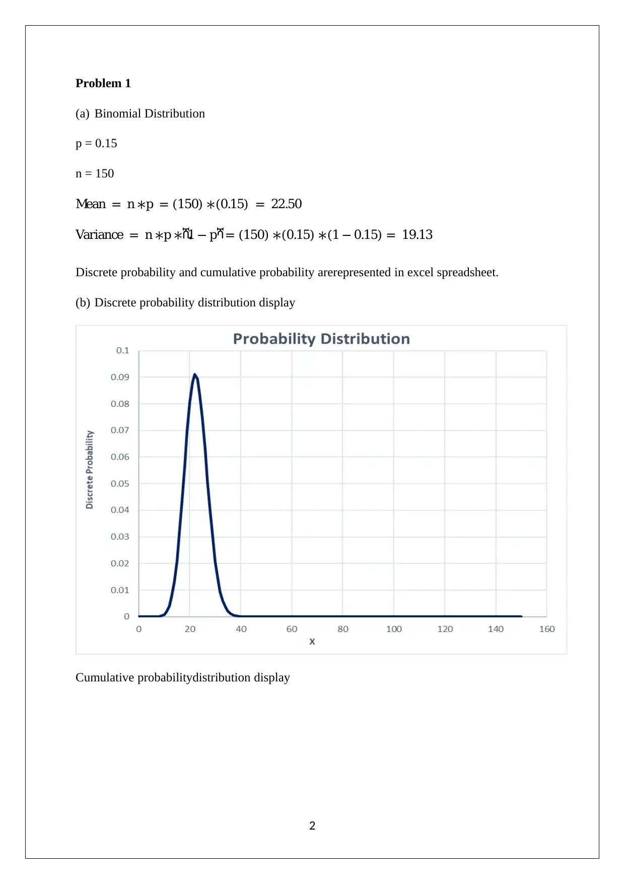
(a) Binomial Distribution
p = 0.15
n = 150
Mean = n ∗p = (150) ∗(0.15) = 22.50
Variance = n ∗p ∗ሺ1 − pሻ= (150) ∗(0.15) ∗(1 − 0.15) = 19.13
Discrete probability and cumulative probability arerepresented in excel spreadsheet.
(b) Discrete probability distribution display
Cumulative probabilitydistribution display
2
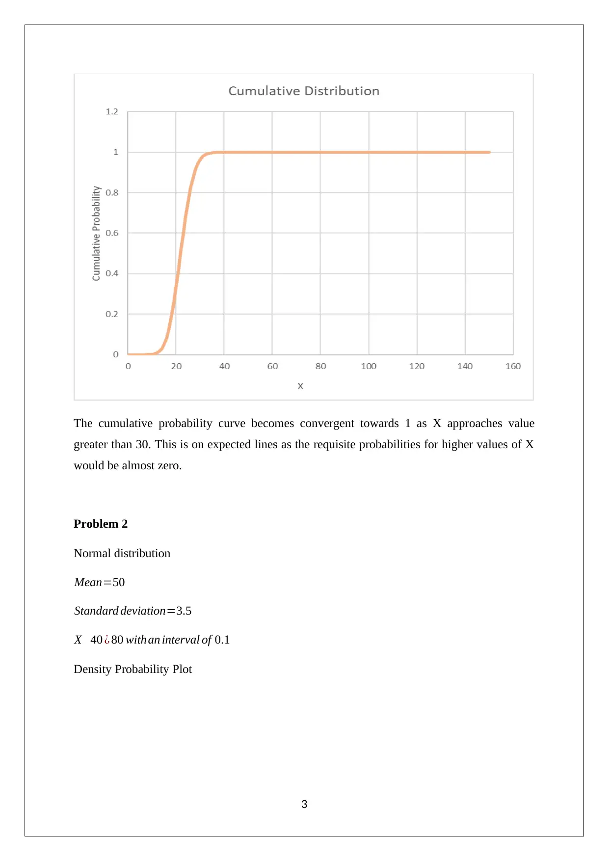
The cumulative probability curve becomes convergent towards 1 as X approaches value
greater than 30. This is on expected lines as the requisite probabilities for higher values of X
would be almost zero.
Problem 2
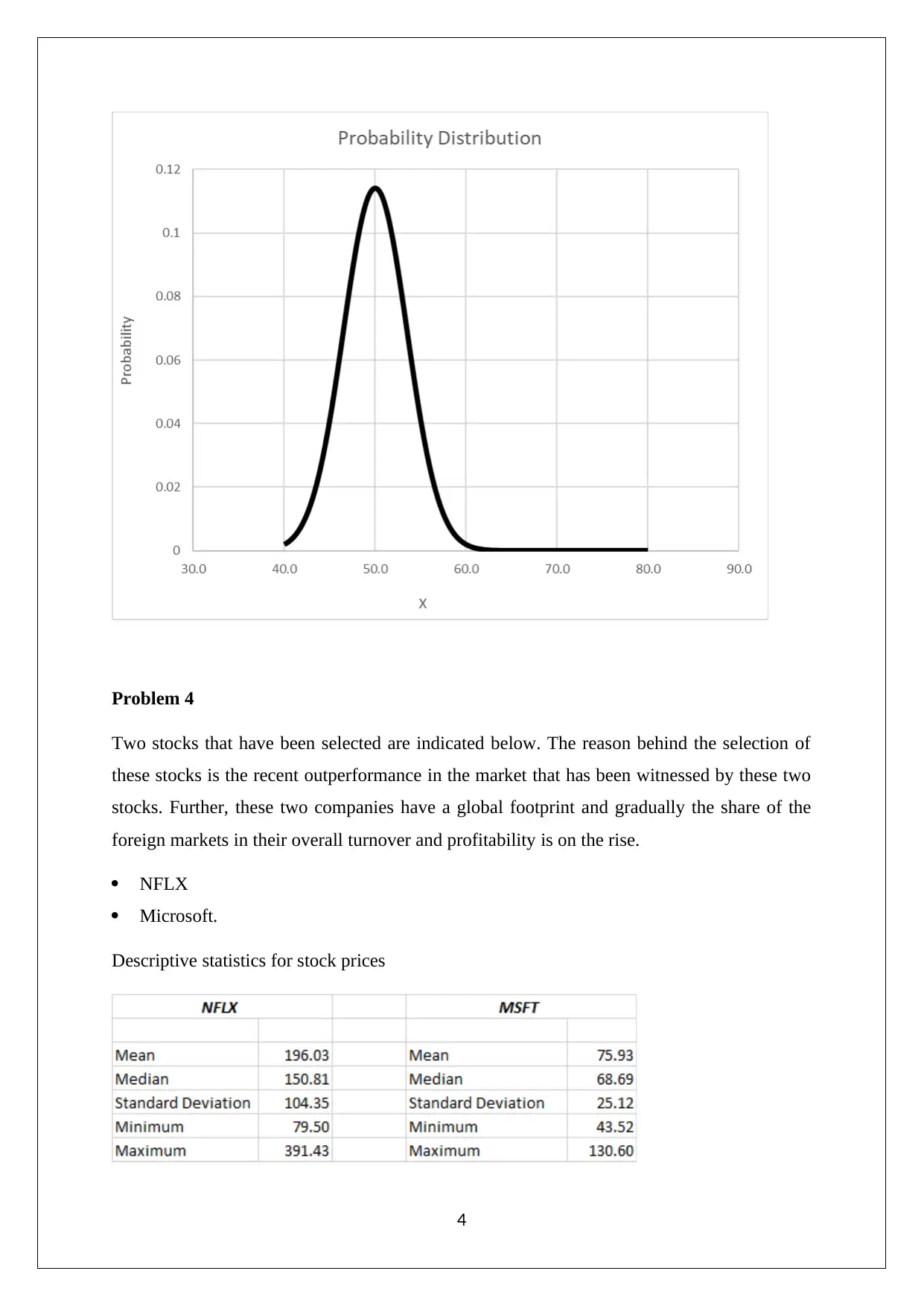
Normal distribution
Mean=50
Standard deviation=3.5
X 40 ¿ 80 withan interval of 0.1
Density Probability Plot
3
greater than 30. This is on expected lines as the requisite probabilities for higher values of X
would be almost zero.
Problem 2
Normal distribution
Mean=50
Standard deviation=3.5
X 40 ¿ 80 withan interval of 0.1
Density Probability Plot
3
⊘ This is a preview!⊘
Do you want full access?
Subscribe today to unlock all pages.

Trusted by 1+ million students worldwide
Problem 4
Two stocks that have been selected are indicated below. The reason behind the selection of
these stocks is the recent outperformance in the market that has been witnessed by these two
stocks. Further, these two companies have a global footprint and gradually the share of the
foreign markets in their overall turnover and profitability is on the rise.
NFLX
Microsoft.
Descriptive statistics for stock prices
4
Paraphrase This Document
Need a fresh take? Get an instant paraphrase of this document with our AI Paraphraser
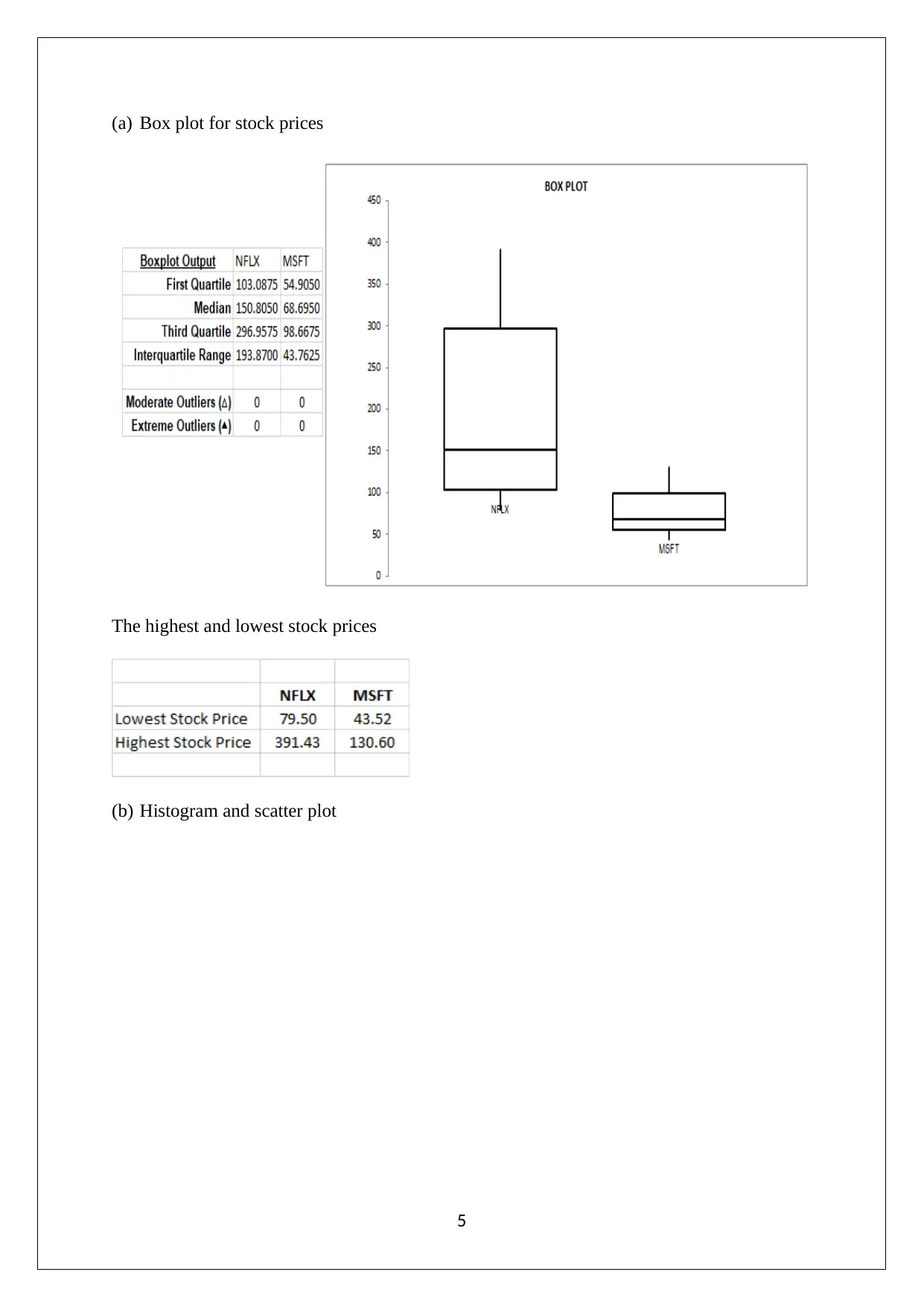
(a) Box plot for stock prices
The highest and lowest stock prices
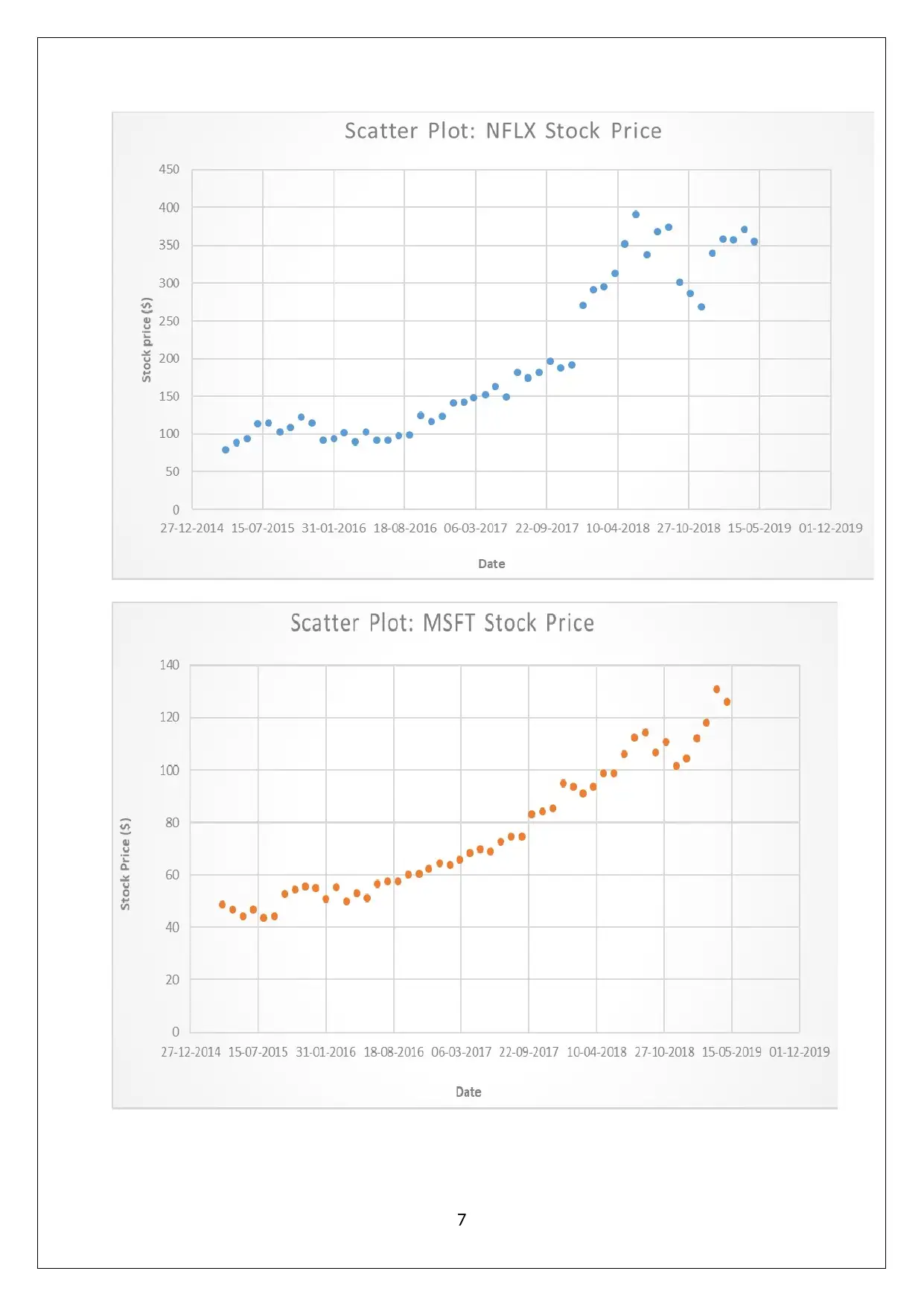
(b) Histogram and scatter plot
5
The highest and lowest stock prices
(b) Histogram and scatter plot
5

6
⊘ This is a preview!⊘
Do you want full access?
Subscribe today to unlock all pages.

Trusted by 1+ million students worldwide
7
Paraphrase This Document
Need a fresh take? Get an instant paraphrase of this document with our AI Paraphraser
c) The comparison of the two box plots highlight that the median prices of the two stocks are
significantly different with Netflix having a higher value. Additionally, the skew present in
the Netflix stock prices also tends to be higher than the corresponding skew present in
Microsoft stock prices. This is primarily because of the recent run up in stock prices where
Netflix has delivered superior returns in comparison to Microsoft.
Problem 5
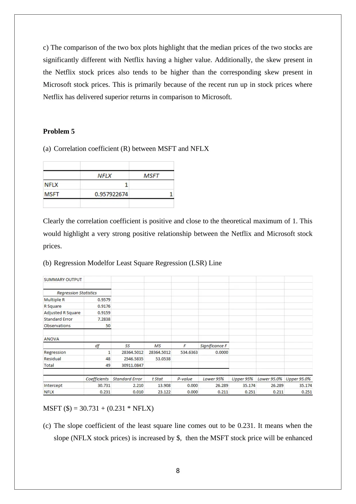
(a) Correlation coefficient (R) between MSFT and NFLX
Clearly the correlation coefficient is positive and close to the theoretical maximum of 1. This
would highlight a very strong positive relationship between the Netflix and Microsoft stock
prices.
(b) Regression Modelfor Least Square Regression (LSR) Line
MSFT ($) = 30.731 + (0.231 * NFLX)
(c) The slope coefficient of the least square line comes out to be 0.231. It means when the
slope (NFLX stock prices) is increased by $, then the MSFT stock price will be enhanced
8
by $0.231. The positive slope implies that the direction of change for both stock prices
would be the same.
(d) In the given regression model, the Microsoft stock price is the dependent variable whose
best value prediction can be derived by the substitution of the median value of the
independent variable i.e. Netflix stock. This is shown below.
MSFT stock price = 30.731 + (0.231 *150.81) = $ 65.57
Problem 6
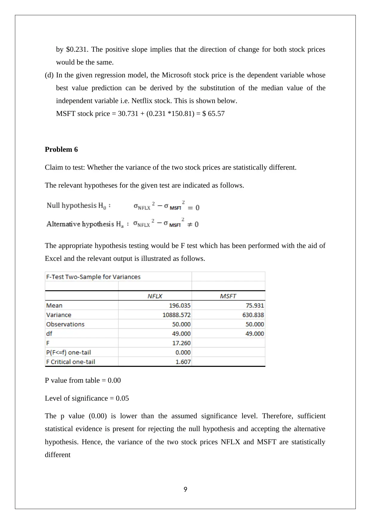
Claim to test: Whether the variance of the two stock prices are statistically different.
The relevant hypotheses for the given test are indicated as follows.
The appropriate hypothesis testing would be F test which has been performed with the aid of
Excel and the relevant output is illustrated as follows.
P value from table = 0.00
Level of significance = 0.05
The p value (0.00) is lower than the assumed significance level. Therefore, sufficient
statistical evidence is present for rejecting the null hypothesis and accepting the alternative
hypothesis. Hence, the variance of the two stock prices NFLX and MSFT are statistically
different
9
⊘ This is a preview!⊘
Do you want full access?
Subscribe today to unlock all pages.

Trusted by 1+ million students worldwide
Problem 7
Claim to test: Stock prices of both stocks are from normal distribution or not.
The relevant hypotheses for the given test are indicated as follows.
H0: The stock price distribution does not deviate significantly from a normal distribution
H1: The stock price distribution does deviate significantly from a normal distribution
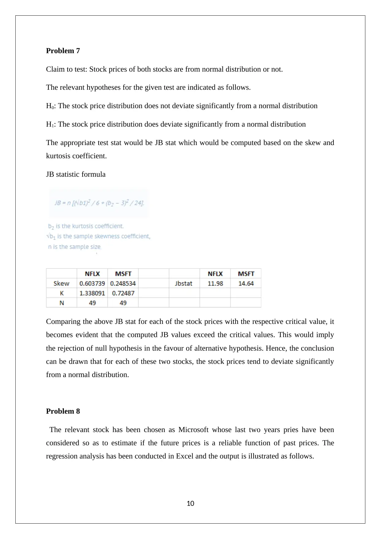
The appropriate test stat would be JB stat which would be computed based on the skew and
kurtosis coefficient.
JB statistic formula
Comparing the above JB stat for each of the stock prices with the respective critical value, it
becomes evident that the computed JB values exceed the critical values. This would imply
the rejection of null hypothesis in the favour of alternative hypothesis. Hence, the conclusion
can be drawn that for each of these two stocks, the stock prices tend to deviate significantly
from a normal distribution.
Problem 8
The relevant stock has been chosen as Microsoft whose last two years pries have been
considered so as to estimate if the future prices is a reliable function of past prices. The
regression analysis has been conducted in Excel and the output is illustrated as follows.
10
Paraphrase This Document
Need a fresh take? Get an instant paraphrase of this document with our AI Paraphraser
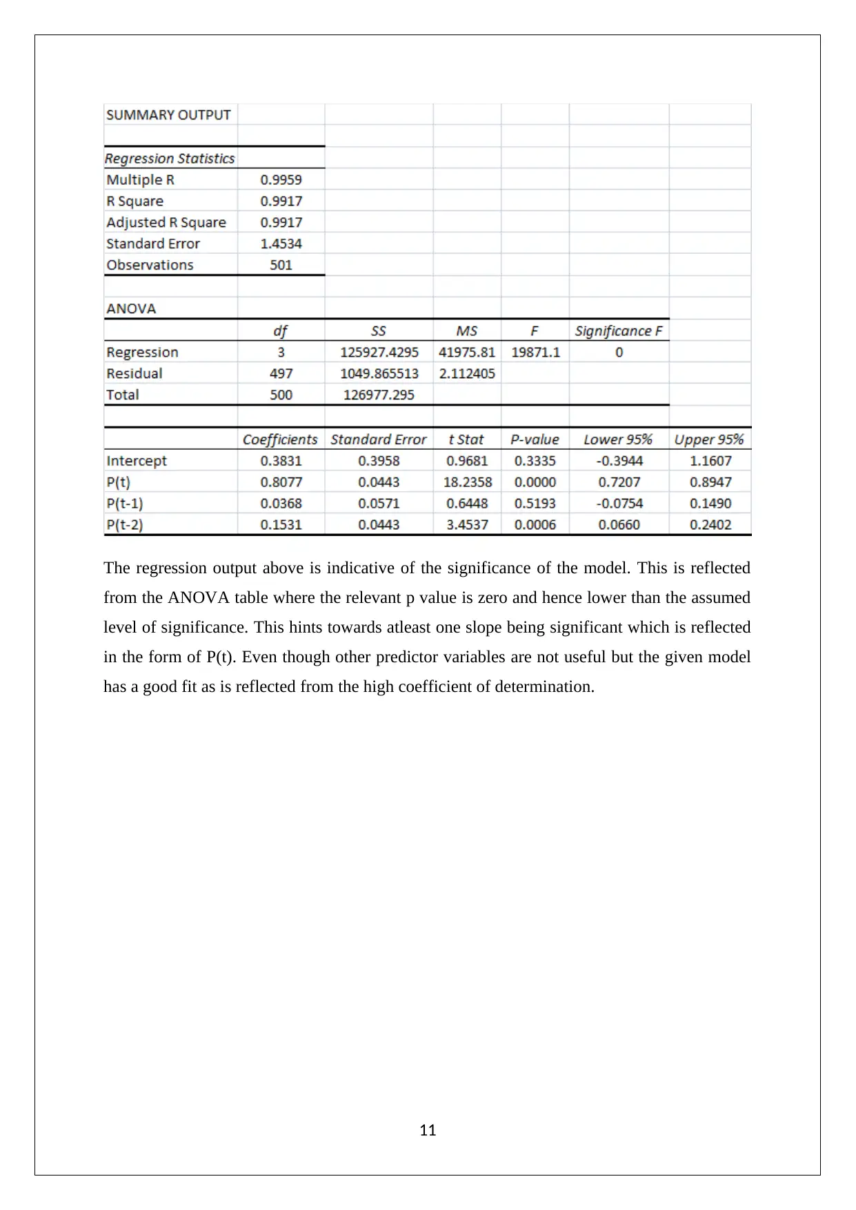
The regression output above is indicative of the significance of the model. This is reflected
from the ANOVA table where the relevant p value is zero and hence lower than the assumed
level of significance. This hints towards atleast one slope being significant which is reflected
in the form of P(t). Even though other predictor variables are not useful but the given model
has a good fit as is reflected from the high coefficient of determination.
11
1 out of 11
Related Documents
Your All-in-One AI-Powered Toolkit for Academic Success.
+13062052269
info@desklib.com
Available 24*7 on WhatsApp / Email
![[object Object]](/_next/static/media/star-bottom.7253800d.svg)
Unlock your academic potential
Copyright © 2020–2026 A2Z Services. All Rights Reserved. Developed and managed by ZUCOL.


