Biostatistics Assignment: STROBE Review & Regression Analysis in R

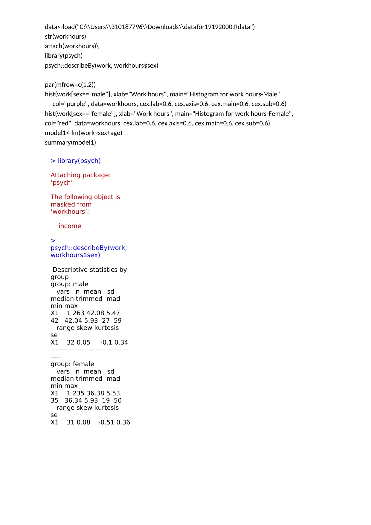
This biostatistics assignment solution includes a critical review of a research paper using selected items from the STROBE checklist, focusing on power analysis, statistical methods, handling of missing data, and reporting of results. It also involves a regression analysis using R Commander to investigate the difference in self-reported work hours between male and female full-time workers in Sydney, controlling for age. The solution provides descriptive statistics, histogram visualizations, regression model results with interpretation, and predictions of work hours for 25-year-old male and female workers, along with the R code used for the analysis. Desklib provides more such solved assignments and study resources for students.

Introduction to Biostatistics
Assignment 2
Statistics
Student Name:
Instructor Name:
Course Number:
2 June 2019

Question 1: Critical review of the paper
In this report, a critical review of the paper by Weston et.al (2019) is presented. The review is based on
items 10, 12-17 of the STROBE checklist. For item 10, it was established that the authors did not mention
anything to do with power analysis, so the author is left wondering whether power analysis was performed
for this study. For item 12, there are 7 items within this subcategory. Review of this items showed that the
authors highlighted items on statistical methods, statistical subgroups, missing data and sampling technique.
The study reported that ordinary least squares (OLS) model was used as the statistical method to perform the
analysis and that multiple imputation was applied to handle the issue of missing data. Analysis was reported
for the subgroups based on gender and that a sample of 11 215 men and 12 188 women was used for this
study. There was however no mention of the sensitivity analysis nor was there report on loss to follow-up as
the study was a cross-sectional study. No reporting was presented for the strobe items 13. This could
because the study used secondary data and as such no explanation for non-participation was required in the
study. For strobe item 14, the study reported on the characteristics of the study participants such as age,
number of children, marital status among others. However, the study did not report on the number of
missing data nor on the follow-up time. No reporting was made for strobe item 15 which is on the number of
events or exposures. All the sub-items within item 16 were reported apart from translation of relative risk to
absolute risk. The study clearly reported on the unadjusted mean depressive symptom estimates for the
temporal work patterns, covariates, and work conditions. The study also reported the confounder adjusted
estimates as well as the 95% confidence interval estimates. The last strobe item (item 17) was also reported.
The interaction of gender was reported in the study. The table below presents the summary of the strobe
items reported in the study.
Strobe item number Item label Reported in the study
(Yes/No)
Item 10 Power analysis No
Item 12 a) Statistical methods Yes
Item 12 b) Statistical subgroups/interactions Yes
Item 12 c) How missing data addressed Yes
Item 12 d) Cohort: How loss to follow up addressed No
Item 12 d) Case control: How matched No
Item 12 d) Cross-sectional: Sampling strategy Yes
Item 12 e) Sensitivity analyses No
Item 13 a) Number at each stage of study No
Item 13 a) Reasons for non-participation No
Item 13 a) Use of flow diagram No
Item 14 a) Characteristics of study participants Yes
Item 14 b) Number with missing data No
Item 14 c) Cohort: Follow-up time No
Item 15 Number of events or exposures No
Item 16 a) Unadjusted estimates Yes
Item 16 a) Confounder adjusted estimates with reasoning Yes
Item 16 a) 95% Confidence Interval Yes
Item 16 b) Category boundaries for continuous variables Yes
Item 16 c) Translate Relative Risk to Absolute Risk No
Item 17 Other analyses
(subgroups/interactions/sensitivity)
Yes

Question 2 (22 marks)
Using R Commander and the data set from the sample of full-time workers in Sydney assigned to you
address the following research questions:
a) By how much do self-reported work hours differ between male and female full-time workers on
average in Sydney after correcting for age? (You should address this question using linear
regression and include associated descriptive analyses.)
Answer
Descriptive statistics
As can be seen in the table below, the average self-reported work hours for the male workers is
42.08 hours with a median of 42.00 hours while that of the female workers is 36.38 hours with a
median of 35.00 hours. The skewness values for the male and female self-reported work hours was
found to be less than 0.5 suggesting that the distribution of the self-reported hours for both the
female and male work hours is approximately normally distributed.
Statistics Sex
Male Female
Mean 42.08 36.38
Standard deviation 5.47 5.53
Median 42.00 35.00
Minimum 27.00 19.00
Maximum 59.00 50.00
Skewness 0.05 0.08
Histogram
The histogram below further confirms that the distribution of self-reported hours for both the
female and male workers is approximately normally distributed (based on the bell-shaped curve).
The results of the regression is presented below;
> model1<-
lm(work~sex+age)
> summary(model1)
Call:

From the above results, we can see that the overall model is significant [F(2, 495) = 66.65, p =
0.000]. The value of R-squared was found to be 0.2122; this implies that 21.22% of the variation in
the self-reported work hours of the employees is explained by the sex of the employee while
controlling for the age of the employee. The variable sex was found to be significant in the model (p
< 0.05) while age was insignificant (p > 0.05)
The coefficient for the dummy variable sex (female = 1, male = 0) was found to be -5.7032; this
implies that a female worker is likely to work (self-reported work hours) for 5.7032 hours less as
compared to the male worker. The intercept coefficient was found to be 42.4492; this implies that
holding sex and age constant we would expect the self-reported hours to be 42.4492 hours.
Based on the above, the estimated regression equation model is thus given as follows;
Workhours=42.4492−5.7032( sexfemale)−0.0092(age)
As can be seen, the self-reported work hours differ by about 5.7032 hours between male and
female full-time workers on average in Sydney after correcting for age. This means that female
workers work for about 5.7032 less time as compared to the male workers.
b) Using the model in a), predict the number of self-reported work hours for 25-year-old male
workers. Repeat for 25-year-old female workers.
Answer
Predicting the number of self-reported work hours for 25-year-old male workers;
Workhours=42.4492−5.7032( sexfemale)−0.0092(age)
Workhours=42.4492−5.7032 ( 0 ) −0.0092 ( 25 )
¿ 42.4492−0.23
¿ 42.2192
Thus the number of self-reported work hours for 25-year-old male worker is 42.2192 hours.
Predicting the number of self-reported work hours for 25-year-old female workers;
Workhours=42.4492−5.7032( sexfemale)−0.0092(age)
Workhours=42.4492−5.7032 ( 1 ) −0.0092 (25 )
¿ 42.4492−5.7032−0.23
¿ 36.516
Thus the number of self-reported work hours for 25-year-old female worker is 36.516 hours.
Appendix
R codes

data<-load("C:\\Users\\310187796\\Downloads\\datafor19192000.Rdata")
str(workhours)
attach(workhours)\
library(psych)
psych::describeBy(work, workhours$sex)
par(mfrow=c(1,2))
hist(work[sex=="male"], xlab="Work hours", main="Histogram for work hours-Male",
col="purple", data=workhours, cex.lab=0.6, cex.axis=0.6, cex.main=0.6, cex.sub=0.6)
hist(work[sex=="female"], xlab="Work hours", main="Histogram for work hours-Female",
col="red", data=workhours, cex.lab=0.6, cex.axis=0.6, cex.main=0.6, cex.sub=0.6)
model1<-lm(work~sex+age)
summary(model1)
> library(psych)
Attaching package:
‘psych’
The following object is
masked from
‘workhours’:
income
>
psych::describeBy(work,
workhours$sex)
Descriptive statistics by
group
group: male
vars n mean sd
median trimmed mad
min max
X1 1 263 42.08 5.47
42 42.04 5.93 27 59
range skew kurtosis
se
X1 32 0.05 -0.1 0.34
-----------------------------------
-----
group: female
vars n mean sd
median trimmed mad
min max
X1 1 235 36.38 5.53
35 36.34 5.93 19 50
range skew kurtosis
se
X1 31 0.08 -0.51 0.36