401077 Biostatistics Assignment 1 Solution: Autumn 2019 Data Analysis

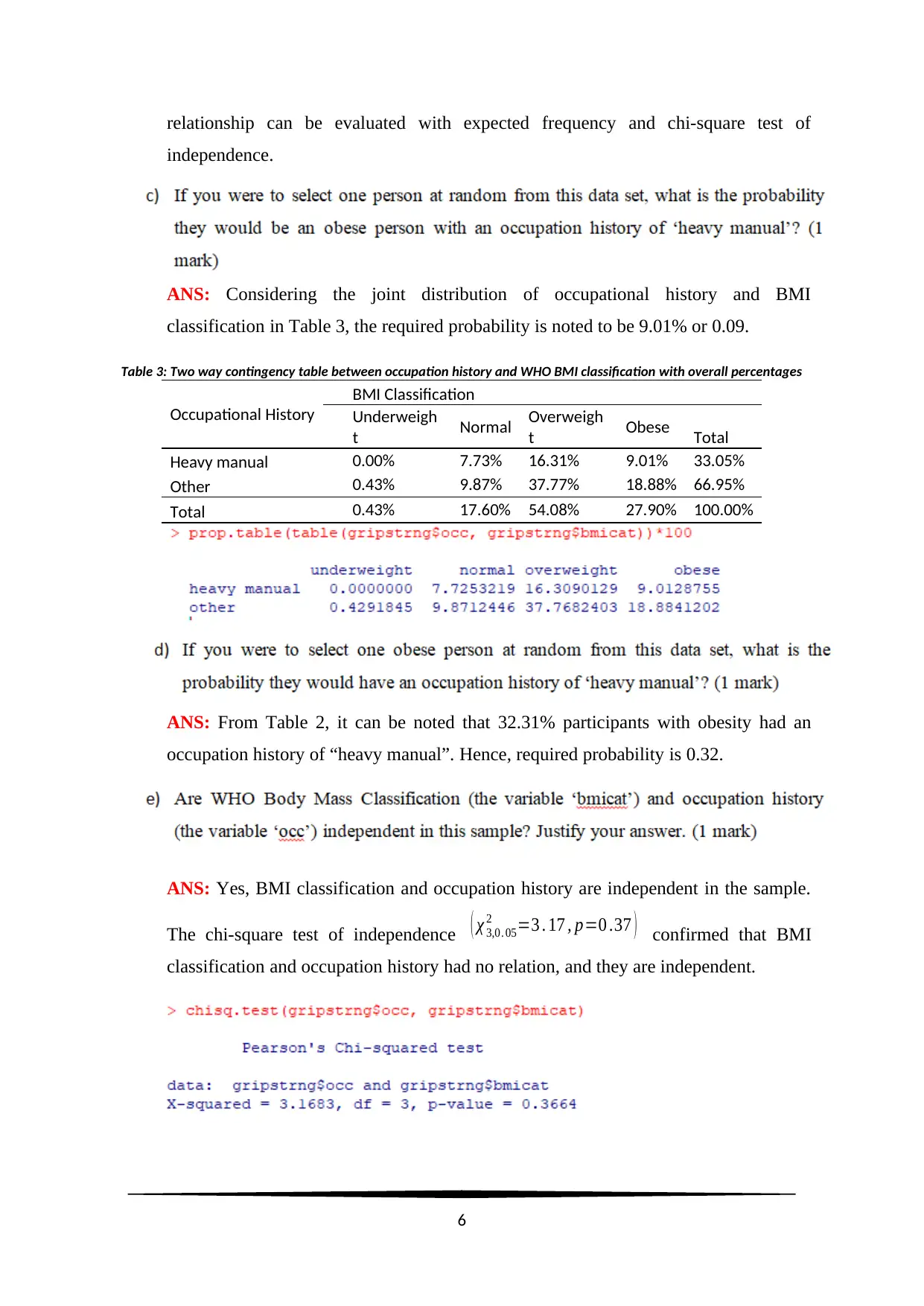
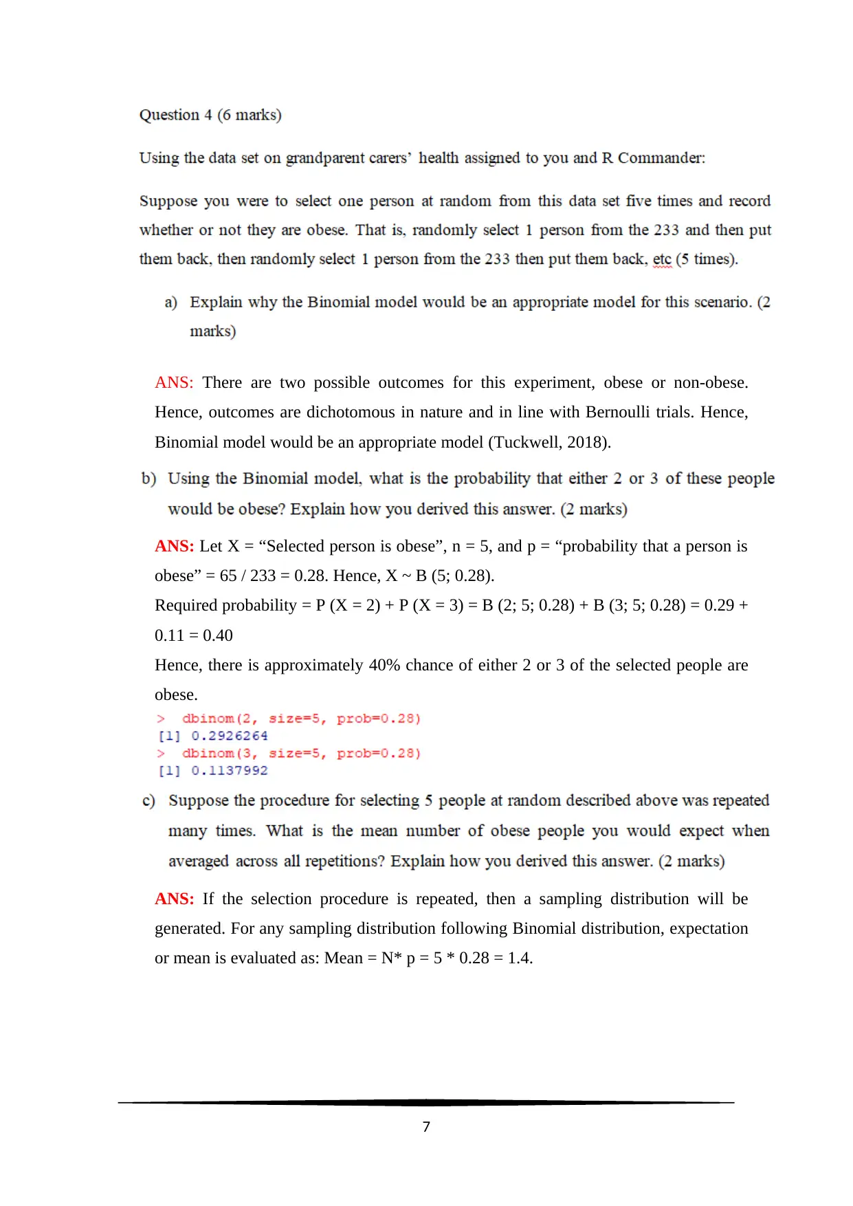
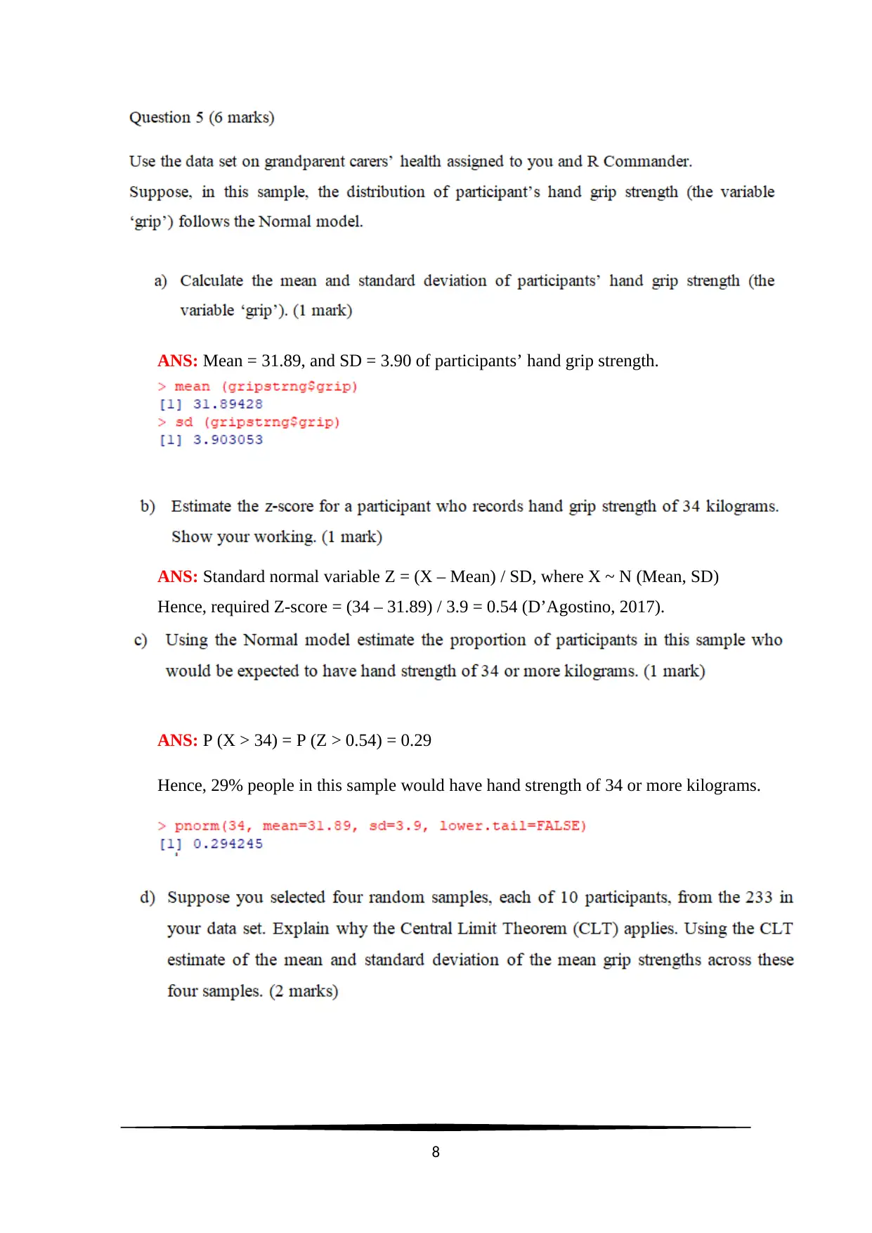
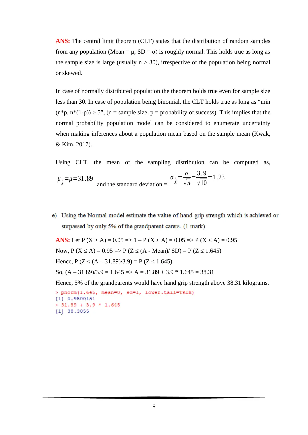
This document presents a comprehensive solution to a biostatistics assignment, focusing on the analysis of a dataset related to the health of grandparent carers. The assignment explores various statistical concepts, including the classification of variables (continuous vs. categorical), descriptive statistics (mean, median, standard deviation), graphical representations (box plots, scatterplots), and inferential statistics (chi-square test, binomial distribution, central limit theorem). The analysis includes the examination of body mass index (BMI), hand grip strength, and occupational history, providing insights into the relationships between these variables. The solution also incorporates the use of R code for data manipulation and analysis, demonstrating practical application of statistical methods. The document addresses questions related to the distribution of BMI, hand grip strength by BMI category, correlation between hand grip strength and BMI, the relationship between occupational history and BMI classification, and the application of binomial distribution and the central limit theorem to the data. The solution includes tables, graphs, and detailed explanations to support the analysis and conclusions.

Introduction to Biostatistics
1

ANS: The variable “grip” is a continuous variable as it is participant’s maximum
hand grip strength in measured in kilograms. Weight is always a continuous variable
and so is “grip”.
Figure 1: WHO body mass classification plot
ANS: WHO body mass classification in Figure 1 reveals that majority (N = 126) of
sample participants are overweight, followed by N = 65 obese participants. Only 1
participant is underweight and 41 are noted to have normal BMI. Hence, majority of
the grandparents participating in the present study are suffering from overweight
hazards.
2

ANS: As measures of central tendency, average BMI is noted to be 28.30 with
median at 27.79. Median is noted to be less than mean, implying the shape of the
distribution to be slightly right skewed. Spread of BMI range of participants is noted
between 17.73 and 40.83, where participants with their BMI in bottom 25% BMI
range is below 25.84. The top 25% BMI of participants is noted above 30.44.
Table 1: Descriptive Summary table of BMI constructed using from R output
Descriptive Summary BMI
Min 17.73
1stQu 25.84
Median 27.79
Mean 28.3
3rdQu 30.44
Max 40.83
ANS: The following side by side box plot in Figure 2 demonstrates the “hand grip
strength” by WHO classification of BMI (Hofmann, Wickham, & Kafadar, 2017).
3

Figure 2: Side by side box plot for Hand grip strength by BMI
The Side-by-side box plot in Figure 2 aids in comparing essential information about
the hand grip strength of participants. The comparison was possible hand grip
strengths for four different levels of BMI indices. Median values and the range of
hand grip strengths are evident from the Side-by-side box plot. It is important to note
that hand grip strength is higher for underweight and then normal BMI classified
people. Overweight and obese are noted to have less hand grip strength compared to
normal and underweight participants. The shape of the hand grip strength is noted to
be normal in “normal” BMI people, whereas, a slight right skewness can be noted for
overweight grandparents. Obese participants are noted to have highly left skewed
distribution of hand grip strength.
ANS: A scatterplot has been drawn to assess the relation between hand grip strength
and BMI of participants.
Figure 3: Scatterplot for Grip strength on BMI
4

Direction and strength of this relationship is noted from the scatterplot in Figure 3,
which reveals that hand grip strength declines with decrease in BMI. Hence, a
negative correlation between hand grip strength and BMI of participants is noted.
However, considering the fact that the data points are scattered randomly, a low
Pearson’s correlation between the two variables is expected.
ANS: The relationship between occupation history of participant and “WHO body
mass classification” has been presented using a two-way contingency table.
Table 2: Two way contingency table of occupation history and WHO BMI classification with column percentages
Occupational History BMI Classification
Underweight Normal Overweight Obese
Heavy manual 0 18 38 21
% 0 43.90% 30.16% 32.31%
Other 1 23 88 44
% 100% 56.10% 69.84% 67.69%
Total 1 41 126 65
ANS: People who had an occupation history as “heavy manuals” are noted to be
considerable less associated with overweight and obesity. However, actual
5

relationship can be evaluated with expected frequency and chi-square test of
independence.
ANS: Considering the joint distribution of occupational history and BMI
classification in Table 3, the required probability is noted to be 9.01% or 0.09.
Table 3: Two way contingency table between occupation history and WHO BMI classification with overall percentages
Occupational History
BMI Classification
Underweigh
t Normal Overweigh
t Obese Total
Heavy manual 0.00% 7.73% 16.31% 9.01% 33.05%
Other 0.43% 9.87% 37.77% 18.88% 66.95%
Total 0.43% 17.60% 54.08% 27.90% 100.00%
ANS: From Table 2, it can be noted that 32.31% participants with obesity had an
occupation history of “heavy manual”. Hence, required probability is 0.32.
ANS: Yes, BMI classification and occupation history are independent in the sample.
The chi-square test of independence ( χ 3,0. 05
2 =3 . 17 , p=0 .37 ) confirmed that BMI
classification and occupation history had no relation, and they are independent.
6

ANS: There are two possible outcomes for this experiment, obese or non-obese.
Hence, outcomes are dichotomous in nature and in line with Bernoulli trials. Hence,
Binomial model would be an appropriate model (Tuckwell, 2018).
ANS: Let X = “Selected person is obese”, n = 5, and p = “probability that a person is
obese” = 65 / 233 = 0.28. Hence, X ~ B (5; 0.28).
Required probability = P (X = 2) + P (X = 3) = B (2; 5; 0.28) + B (3; 5; 0.28) = 0.29 +
0.11 = 0.40
Hence, there is approximately 40% chance of either 2 or 3 of the selected people are
obese.
ANS: If the selection procedure is repeated, then a sampling distribution will be
generated. For any sampling distribution following Binomial distribution, expectation
or mean is evaluated as: Mean = N* p = 5 * 0.28 = 1.4.
7

ANS: Mean = 31.89, and SD = 3.90 of participants’ hand grip strength.
ANS: Standard normal variable Z = (X – Mean) / SD, where X ~ N (Mean, SD)
Hence, required Z-score = (34 – 31.89) / 3.9 = 0.54 (D’Agostino, 2017).
ANS: P (X > 34) = P (Z > 0.54) = 0.29
Hence, 29% people in this sample would have hand strength of 34 or more kilograms.
8

ANS: The central limit theorem (CLT) states that the distribution of random samples
from any population (Mean = μ, SD = σ) is roughly normal. This holds true as long as
the sample size is large (usually n > 30), irrespective of the population being normal
or skewed.
In case of normally distributed population the theorem holds true even for sample size
less than 30. In case of population being binomial, the CLT holds true as long as “min
(n*p, n*(1-p)) > 5”, (n = sample size, p = probability of success). This implies that the
normal probability population model can be considered to enumerate uncertainty
when making inferences about a population mean based on the sample mean (Kwak,
& Kim, 2017).
Using CLT, the mean of the sampling distribution can be computed as,
μX
¿ =μ=31 .89 and the standard deviation =
σ X
¿ = σ
√ n = 3 . 9
√ 10 =1 .23
ANS: Let P (X > A) = 0.05 => 1 – P (X ≤ A) = 0.05 => P (X ≤ A) = 0.95
Now, P (X ≤ A) = 0.95 => P (Z ≤ (A - Mean)/ SD) = P (Z ≤ 1.645)
Hence, P (Z ≤ (A – 31.89)/3.9) = P (Z ≤ 1.645)
So, (A – 31.89)/3.9 = 1.645 => A = 31.89 + 3.9 * 1.645 = 38.31
Hence, 5% of the grandparents would have hand grip strength above 38.31 kilograms.
9

References
D’Agostino, R. B. (2017). Tests for the normal distribution. In Goodness-of-fit-techniques
(pp. 367-420). Routledge.
Hofmann, H., Wickham, H., & Kafadar, K. (2017). Value plots: Boxplots for large data.
Journal of Computational and Graphical Statistics, 26(3), 469-477.
Kwak, S. G., & Kim, J. H. (2017). Central limit theorem: the cornerstone of modern
statistics. Korean journal of anesthesiology, 70(2), 144.
Tuckwell, H. (2018). Elementary applications of probability theory (2nd ed.). New York:
Routledge.
10

Appendices – R-Codes
ls ()
summary (gripstrng$bmi)
plot(gripstrng$bmicat,xlab="BMI Category",ylab="Frequency",col="blue",
main="BMI Category Distribution chart",args.legend=list(bty="n",horiz=TRUE)
border="red")
boxplot(grip ~ bmicat, data = gripstrng, xlab = “BMI Category”, ylab = “Hand grip strength
in kilograms”, main = "BMI Category wise Participant’s maximum hand grip strength")
plot(gripstrng$grip ~ gripstrng$bmi, xlab = " Body Mass Index ",
ylab = "Hand grip strength in kilograms ",
main = "Maximum hand grip strength on BMI"
)
table(gripstrng$occ, gripstrng$bmicat)
prop.table(table(gripstrng$occ, gripstrng$bmicat), margin = 2)*100
chisq.test(gripstrng$occ, gripstrng$bmicat)
dbinom(2, size=5, prob=0.28)
dbinom(3, size=5, prob=0.28)
pnorm(34, mean=31.89, sd=3.9, lower.tail=FALSE)
pnorm(1.645, mean=0, sd=1, lower.tail=TRUE)
11