Autumn 2018 Biostatistics 401077 Assignment 3: STROBE Checklist Review

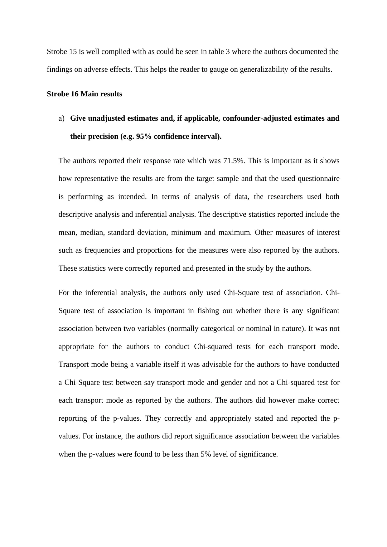
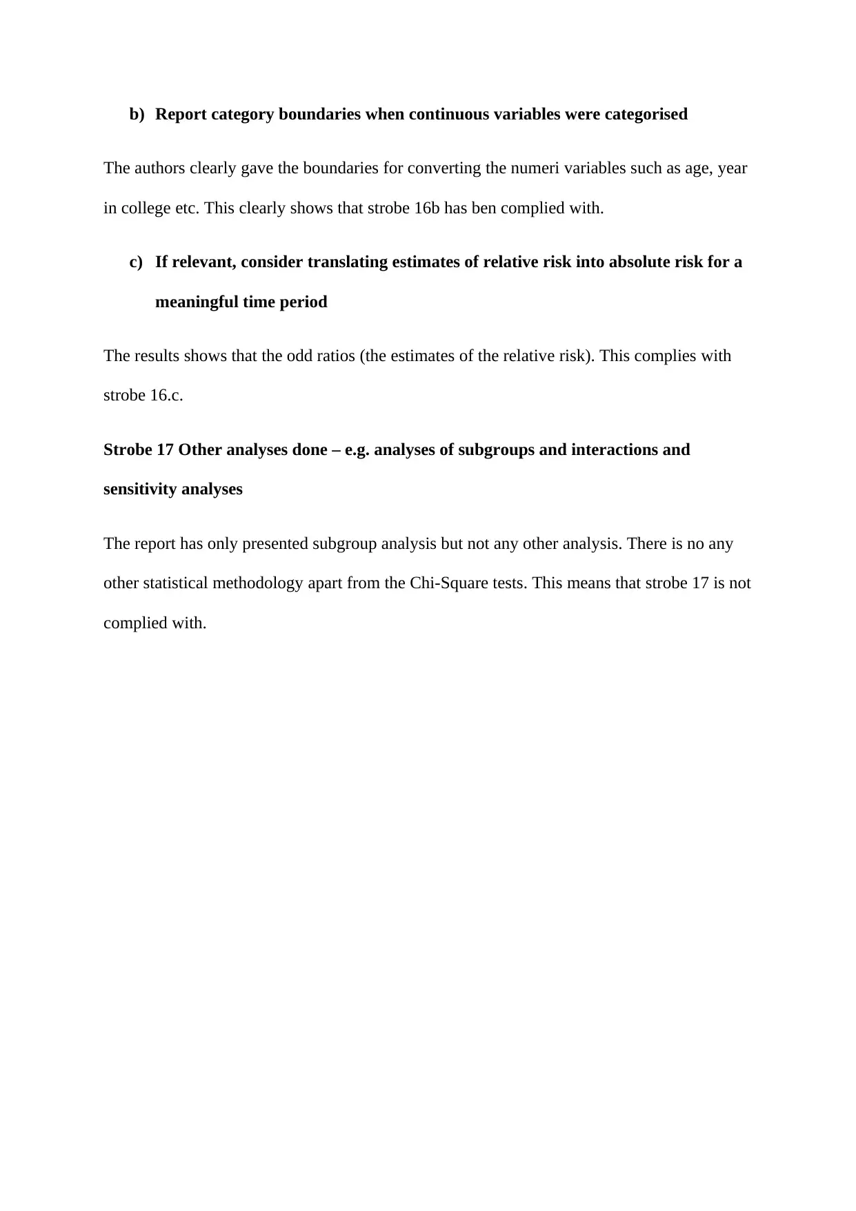
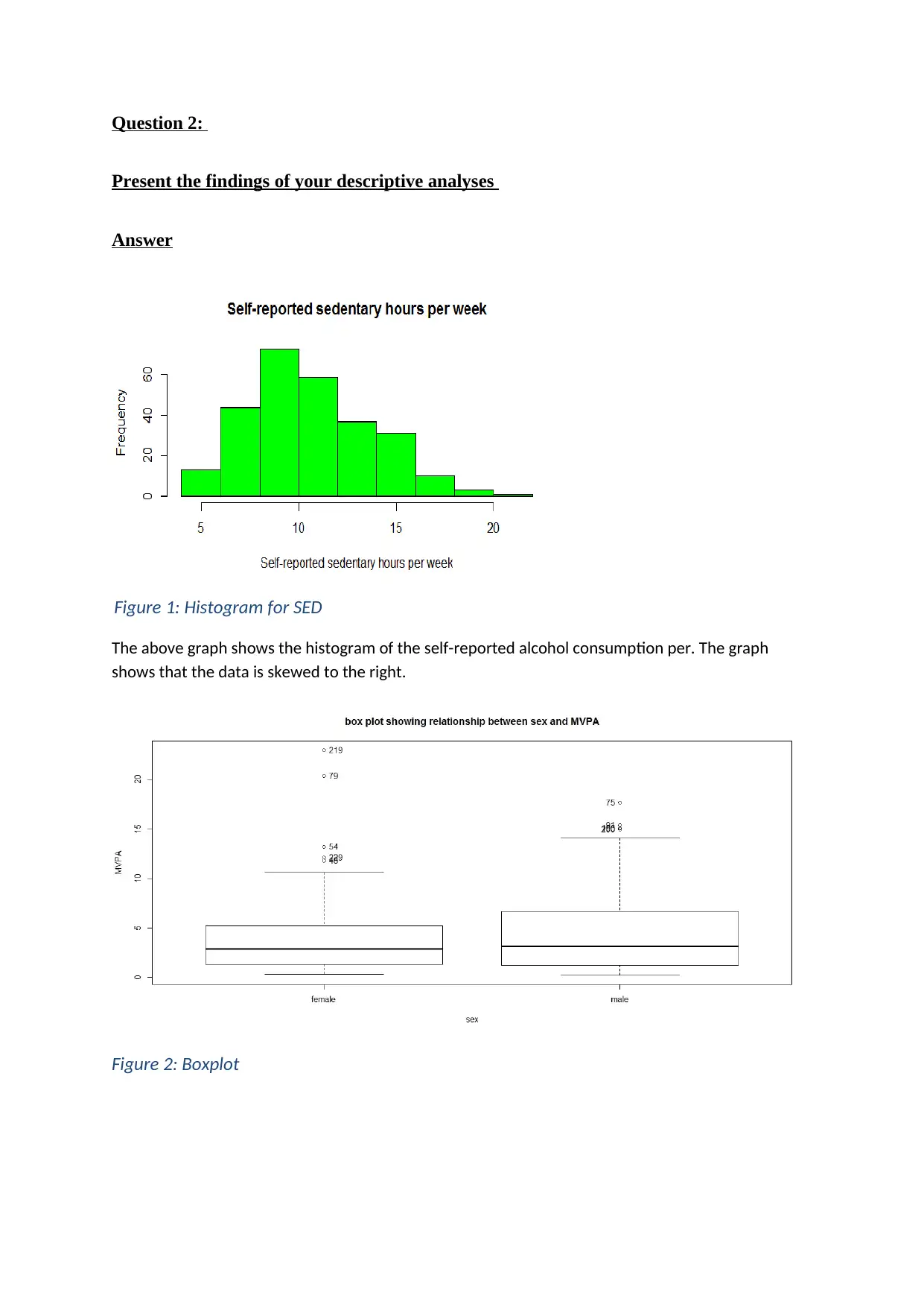
This document presents a comprehensive solution to a biostatistics assignment, focusing on a critical appraisal of a research paper using the STROBE checklist. The assignment involves a 400-500 word report evaluating the statistical material in the paper against items 10, 12-17 of the STROBE checklist. The student analyzed the paper's adherence to the checklist, highlighting strengths and weaknesses in the documentation of statistical methods. The assignment also includes descriptive analyses, such as histograms and boxplots, and inferential analyses, including t-tests and regression models, to address research questions related to the mean MVPA of male and female participants and the factors influencing logMVPA. The results revealed no significant difference in mean MVPA between genders, but found that self-reported sedentary hours significantly influenced logMVPA. The document includes the student's analysis, findings, and interpretations, along with relevant code and output from statistical software.

401077 Introduction to Biostatistics, Autumn 2018
Assignment 3
Due Sunday November 4, 2018
Student name:
Student number:

Task 1:
Critically appraise of the statistical material in this paper against items 10, 12-17 of the
STROBE checklist. Present your review as a 400-500 word report.
Strobe 10 Study size
The authors have clearly stated the sample size used and they used a sample size of 775. This
sample size is big enough to warrant significant statistical results.
Strobe 12 Statistical methods
a) Describe all statistical methods, including those used to control for confounding
In terms of the statistical methods used, the authors failed to mention the statistical methods
they used. For instance, the report does not mention the descriptive analysis performed nor
the inferential statistics. However, the authors have just presented the results. I was able to
pick out Chi-Square test as having been used by the authors to test for the association
between variables.
No mention of adjustment of possible confounders by the authors. So in short, the authors
have failed to adhere with strobe 12a requirements. This requirements needs the authors to
document the statistical methods used and why.
b) Describe any methods used to examine subgroups and interactions
The authors did not mention the methodology of analysing the subgroups. However, in the
results section presented in tables 1, 2 and 3, the authors report the subgroups of male and
female separately as well as those of different age groups. This was not however mentioned
in the statistical methods. This means that item 12b was not complied with.
c) Explain how missing data were addressed

The authors did not mention about how they went about dealing with the missing data. The
results shows that there is evidence of missing data, however, this is not acknowledged
anywhere in the report. It is therefore difficult for the reader to ascertain the level of bias that
could arise as a result of the missing data. In conclusion the authors failed to comply with
item 12c of the strobe.
d) Cross-sectional study – if applicable, describe analytical methods taking account
for sampling strategy
From the study process, this was a cross-sectional study. The authors adequately addressed
how the sampling was done thereby addressing item 12d of the strobe. However, the readers
are left wondering why the data collection was restricted to some days of the week only. This
could potentially result to bias in the results.
e) Describe any sensitivity analyses
The authors did not mention anything to do with sensitivity analysis.
Strobe 13: Participants
a) Report number of individuals at each stage of study – eg numbers potentially eligible,
examined for eligibility, confirmed eligible, included in the study, completing follow-
up and analyses
The authors did mention the proportion of participants in the study. They gave the number of
lecturers and students involved in the study-this is in compliance with strobe 12a. However,
there was no breakdown of those who dropped from the study.
b) Give reasons for non-participant at each stage

The authors did not give the reasons for non-participant-this is not documented anywhere in
the study. This clearly violates strobe 13b.
c) Consider use of a flow diagram
There is no flow diagram indicating the response. Even though this is not a major risk to bias
by the reader, it is in contraction with Strobe 13c.
Strobe 14 Descriptive data
a) Give characteristics of study participants (e.g. demographic, clinical , social) and
information on exposures and potential confounders
Table 1 gives the descriptive statistics of the study participants. For instance, it gives the
proportion of female and male participants in the study as well as their ages, ethnicity and
income.
b) Indicate number of participants with missing data for each variable of interest
Strobe 14b has not been complied with by the authors as could be seen in the report. There
are some missing data but the authors did not mention h=on how the missing data was
handled. Failure to acknowledge the missing data is wrong since the reader is not informed of
potential bias and how this was mitigated.
c) Cohort study: Summarise follow-up time – e.g. average and total amount.
Strobe 14c is irrelevant in this study based on the fact that this is a cross-sectional survey.
Strobe 15
Cross-sectional study—Report numbers of outcome events or summary measures

Strobe 15 is well complied with as could be seen in table 3 where the authors documented the
findings on adverse effects. This helps the reader to gauge on generalizability of the results.
Strobe 16 Main results
a) Give unadjusted estimates and, if applicable, confounder-adjusted estimates and
their precision (e.g. 95% confidence interval).
The authors reported their response rate which was 71.5%. This is important as it shows
how representative the results are from the target sample and that the used questionnaire
is performing as intended. In terms of analysis of data, the researchers used both
descriptive analysis and inferential analysis. The descriptive statistics reported include the
mean, median, standard deviation, minimum and maximum. Other measures of interest
such as frequencies and proportions for the measures were also reported by the authors.
These statistics were correctly reported and presented in the study by the authors.
For the inferential analysis, the authors only used Chi-Square test of association. Chi-
Square test of association is important in fishing out whether there is any significant
association between two variables (normally categorical or nominal in nature). It was not
appropriate for the authors to conduct Chi-squared tests for each transport mode.
Transport mode being a variable itself it was advisable for the authors to have conducted
a Chi-Square test between say transport mode and gender and not a Chi-squared test for
each transport mode as reported by the authors. The authors did however make correct
reporting of the p-values. They correctly and appropriately stated and reported the p-
values. For instance, the authors did report significance association between the variables
when the p-values were found to be less than 5% level of significance.

b) Report category boundaries when continuous variables were categorised
The authors clearly gave the boundaries for converting the numeri variables such as age, year
in college etc. This clearly shows that strobe 16b has ben complied with.
c) If relevant, consider translating estimates of relative risk into absolute risk for a
meaningful time period
The results shows that the odd ratios (the estimates of the relative risk). This complies with
strobe 16.c.
Strobe 17 Other analyses done – e.g. analyses of subgroups and interactions and
sensitivity analyses
The report has only presented subgroup analysis but not any other analysis. There is no any
other statistical methodology apart from the Chi-Square tests. This means that strobe 17 is not
complied with.

Question 2:
Present the findings of your descriptive analyses
Answer
The above graph shows the histogram of the self-reported alcohol consumption per. The graph
shows that the data is skewed to the right.
Figure 2: Boxplot
Figure 1: Histogram for SED

Figure 2 above shows the boxplot for the self-reported sedentary hours per week. As can be
seen, there two groups do not seem to have a normally distributed data for the SED. There are
also presence of outliers in the dataset as can be seen from the plots.
A bar chart was plotted to visualize on the type of transport used by the participants. As can
be seen in figure 1 below, majority used passenger bus (45.4%, n = 123) as a means of
transport. Those who drove themselves were the second majority (29.5%, n = 80). Those who
used other means of transport were represented by (25.1%, n = 68).
Figure 3: Transport type
Another bar chart was plotted to visualize on the type of licence possessed by the
participants. As can be seen in figure 2 below, majority used passenger bus (45.4%, n = 123)
as a means of transport. Those who drove themselves were the second majority (29.5%, n =
80). Those who used other means of transport were represented by (25.1%, n = 68).

Figure 4: licence type
Not licenced Learners
permit
licenced
counts 69 75 127
driver Passenger Other
counts 80 123 68
Present the findings of relevant regression models and inferential analyses
Is there significant difference between the average MVPA for the male and female
participants?
The following hypothesis was tested;
H0 : μm=μf
H A : μm ≠ μf
This was tested at 5% level of significance.
The results are provided below;

As can be seen, the p-value is 0.1473 (a value greater than 5% level of significance), the null
hypothesis is therefore not rejected and we conclude that the mean MVPA is not different for
the male and female participants.
Regression analysis
We fitted a linear regression model that sought to predict the logMVPA based on the
respondents self-reported sedentary hours per week (sed), number of activities attended in the
past month (activities) and dummy variable for the male.
> t.test(MVPA~sex)
Welch Two Sample t-test
data: MVPA by sex
t = -1.4535, df = 268.98, p-value = 0.1473
alternative hypothesis: true difference in means is not equal to 0
95 percent confidence interval:
-1.6225873 0.2443422
sample estimates:
mean in group female mean in group male
3.857031 4.546154
> fit <- lm(logMVPA ~
sed + activities + sex,
data=survey)
> summary(fit) # show
results
Call:
lm(formula = logMVPA ~
sed + activities + sex,
data = survey)
Residuals:
Min 1Q Median
3Q Max
-1.08251 -0.27316
0.02966 0.32876
0.83822
Coefficients:
Estimate Std.
Error t value Pr(>|t|)
(Intercept) 0.770529
0.285023 2.703
0.007304 **
sed -0.039924
0.010921 -3.656
0.000309 ***

The value of R-Squared is 0.096; this means that only 9.6% of the variation in the dependent
variable (logMVPA) is explained by the three independent variables in the model. The
remaining close to 90% of the variation is explained by factors outside the model (error
term).
The model was however found to be significant when it comes to predicting the applications
(F(3,96) = 17.102, p = 0.000).
Out of the three independent variables only one (sed) was found to be significant in the
model.
 The coefficient for the sed is -0.04; this means that a unit increase in the respondents self-
reported sedentary hours per week would result to the logMVPA decreasing by 0.04.
Similarly, a unit decrease in the respondents self-reported sedentary hours per week
would result to the logMVPA increasing by 0.04.
Considering the significant independent variable only, we the regression model constructed
as follows;
logMVPA=0.77−0.04 (sed )
Provide your answer to the research question
The first research question sought to find out whether there is significant difference in the
mean MVPA for the male and female participants. Results showed that mean MVPA is not
different for the male and female participants.
The second research question sought to determine the significant factors that influence the
logMVPA. Results showed that only one variable (respondents self-reported sedentary hours
per week) significantly influences the change in logMVPA.

Appendix
head(survey)
attach(survey)
boxplot(sed~sex,data=mtcars, main="Self-reported sedentary hours per week"
, ylab="SED", col="green")
hist(sed,data=mtcars, main="Self-reported sedentary hours per week"
, xlab="Self-reported sedentary hours per week", ylab="Frequency", col="green")
counts1 <- table(licence)
barplot(counts, main="Bar chart of licence type",
xlab="Licence Type", col=c("grey","blue", "purple"))
counts1
counts2 <- table(transport)

barplot(counts, main="Bar chart of transport type",
xlab="Transport Type", col=c("darkblue","red", "green"))
counts2
t.test(MVPA~sex)
fit <- lm(logMVPA ~ sed + activities + sex, data=survey)
summary(fit) # show results