University of Eastern Sydney: 401077 Biostatistics Assignment 1

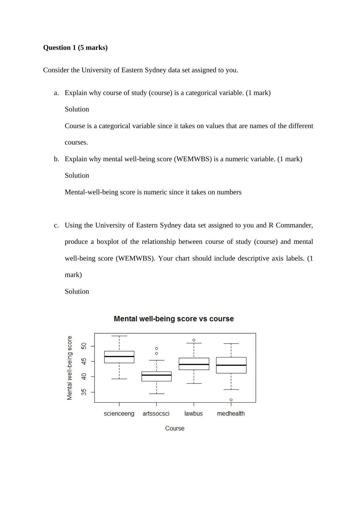
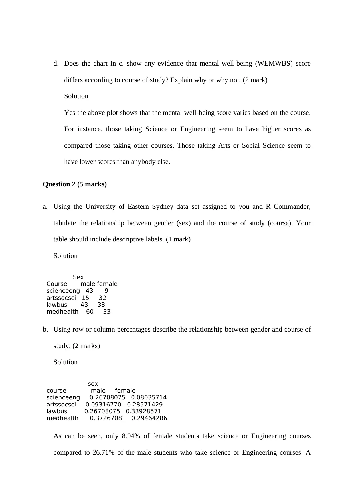
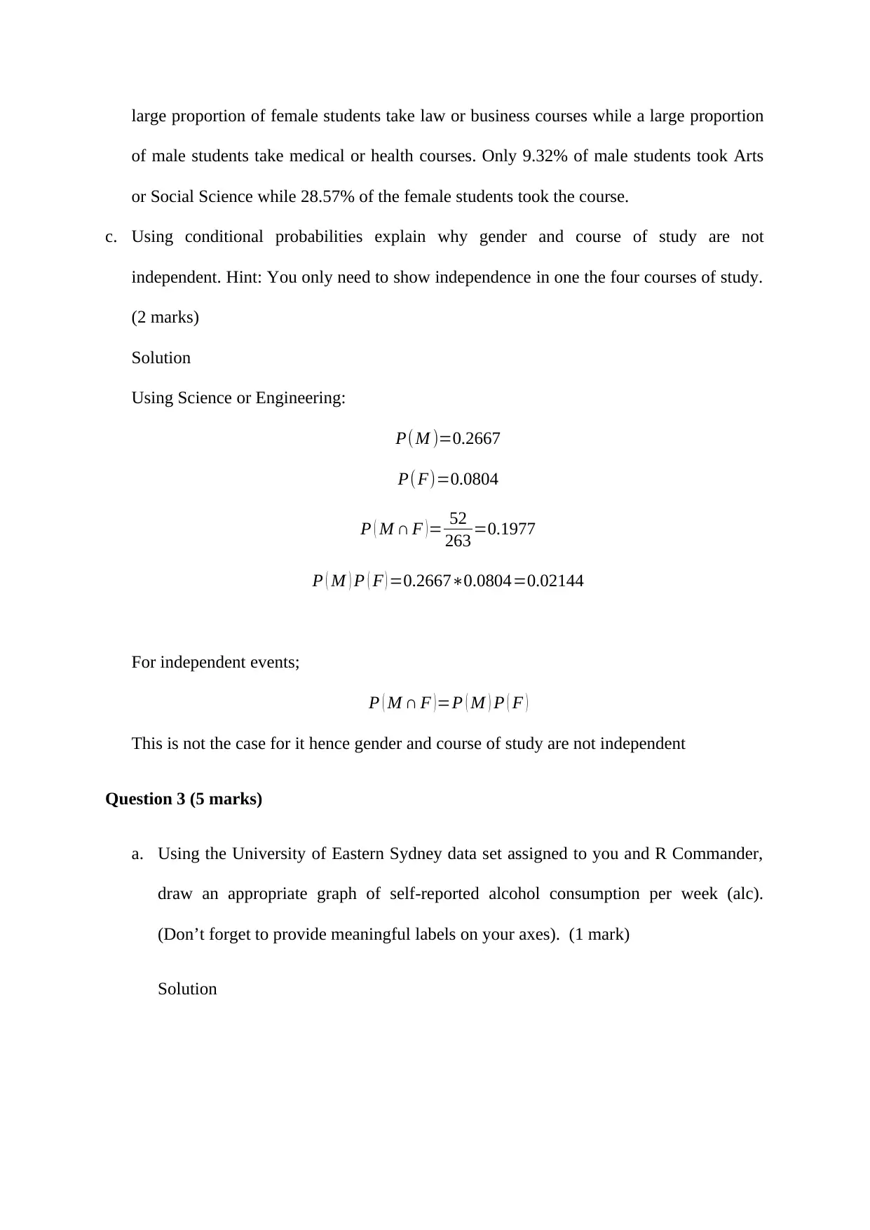
This assignment is a comprehensive analysis of a biostatistics dataset from the University of Eastern Sydney. It begins by exploring categorical and numeric variables, specifically course of study and mental well-being scores, using boxplots to visualize their relationship. The assignment then delves into the relationship between gender and course of study, using tables and percentages to describe the data, and explaining independence using conditional probabilities. Further, the assignment analyzes self-reported alcohol consumption through histograms and statistical measures of shape, center, and spread. It also examines the relationship between log-transformed alcohol consumption and mental well-being scores using scatterplots. The assignment then addresses probability questions related to alcohol consumption and the normal distribution of mental well-being scores, utilizing the central limit theorem. Finally, the assignment explores the sufficiency of given information to determine probabilities and interprets Z-scores to assess the likelihood of needing treatment for depression and anxiety. R codes are provided for the analysis.

401077 Introduction to Biostatistics, Autumn 2018
Assignment 1
Due Sunday April 1, 2018

Question 1 (5 marks)
Consider the University of Eastern Sydney data set assigned to you.
a. Explain why course of study (course) is a categorical variable. (1 mark)
Solution
Course is a categorical variable since it takes on values that are names of the different
courses.
b. Explain why mental well-being score (WEMWBS) is a numeric variable. (1 mark)
Solution
Mental-well-being score is numeric since it takes on numbers
c. Using the University of Eastern Sydney data set assigned to you and R Commander,
produce a boxplot of the relationship between course of study (course) and mental
well-being score (WEMWBS). Your chart should include descriptive axis labels. (1
mark)
Solution

d. Does the chart in c. show any evidence that mental well-being (WEMWBS) score
differs according to course of study? Explain why or why not. (2 mark)
Solution
Yes the above plot shows that the mental well-being score varies based on the course.
For instance, those taking Science or Engineering seem to have higher scores as
compared those taking other courses. Those taking Arts or Social Science seem to
have lower scores than anybody else.
Question 2 (5 marks)
a. Using the University of Eastern Sydney data set assigned to you and R Commander,
tabulate the relationship between gender (sex) and the course of study (course). Your
table should include descriptive labels. (1 mark)
Solution
Sex
Course male female
scienceeng 43 9
artssocsci 15 32
lawbus 43 38
medhealth 60 33
b. Using row or column percentages describe the relationship between gender and course of
study. (2 marks)
Solution
sex
course male female
scienceeng 0.26708075 0.08035714
artssocsci 0.09316770 0.28571429
lawbus 0.26708075 0.33928571
medhealth 0.37267081 0.29464286
As can be seen, only 8.04% of female students take science or Engineering courses
compared to 26.71% of the male students who take science or Engineering courses. A

large proportion of female students take law or business courses while a large proportion
of male students take medical or health courses. Only 9.32% of male students took Arts
or Social Science while 28.57% of the female students took the course.
c. Using conditional probabilities explain why gender and course of study are not
independent. Hint: You only need to show independence in one the four courses of study.
(2 marks)
Solution
Using Science or Engineering:
P( M )=0.2667
P( F)=0.0804
P ( M ∩ F )= 52
263 =0.1977
P ( M ) P ( F ) =0.2667∗0.0804=0.02144
For independent events;
P ( M ∩ F )=P ( M ) P ( F )
This is not the case for it hence gender and course of study are not independent
Question 3 (5 marks)
a. Using the University of Eastern Sydney data set assigned to you and R Commander,
draw an appropriate graph of self-reported alcohol consumption per week (alc).
(Don’t forget to provide meaningful labels on your axes). (1 mark)
Solution

b. Describe the shape of this distribution of self-reported alcohol consumption. Include
appropriate numerical measures (statistics) of shape in your description. (2 marks)
Solution
The above histogram shows that the distribution of data is skewed to the right (longer
tail to the right). It also shows that majority took an average of 10 alcohol
consumption per week measured in standard drinks.
c. Using appropriate statistics describe the centre and spread of the distribution of the
students’ self-reported average alcohol consumption. You must differentiate which
result(s) apply to centre and which apply to spread. (2 marks)
Solution
Min. 1st Qu. Median Mean 3rd Qu. Max. Sd.
0.500 1.000 5.000 9.075 11.000 90.000 12.01886
As can be seen, the average self-reported alcohol consumption is 9.075 with a median
value being 5. On the other hand the standard deviation is 12.02; this shows that the
data is widely distributed. Mean and median are applied to centre while standard
deviation is applied to spread.
Question 4 (4 marks)

a. Using the University of Eastern Sydney data set assigned to you and R Commander,
graph the relationship between the logarithm transformed self-reported alcohol
consumption (logalc) and mental wellbeing (WEMWBS) score. (1 mark)
Solution
b. Describe in words the relationship between log alcohol consumption per week and
mental well-being (WEMWBS) score in this data set. (3 marks)
Solution
From the above graph, it seems there is a negative relationship between log alcohol
consumption per week and mental well-being (WEMWBS) score. This means that an
increase in logalc results to a decrease in WEMWBS while a decrease in logalc results
to an increase in WEMWBS.

Question 5 (3 marks)
In Ireland, Davoren et el (2015) report that that 65.2% of male University students self-
reported alcohol consumption levels which are classified as hazardous.
A random sample of 30 Australian male university students were interviewed about their
alcohol consumption.
a. If Australian male university student do not differ from the Irish male university students,
what is the probability that our random sample of 30 Australian male students will
contain 15 or less students with hazardous alcohol consumption levels? (1 mark)
Solution
P= 20
161 =0.1242=12.42 %
b. If Australian male university students do not differ from the Irish male university
students, we would predict 25% of all samples to contain fewer than how many students
with hazardous alcohol consumption? (1 mark)
Solution
From the data, 20 students had hazardous alcohol consumption
c. If Australian male university students do not differ from the Irish male university
students, estimate the mean number of students with hazardous alcohol consumption per
sample of size 30 males? Show any working. (1 mark)
Solution
Mean=np=30∗0.1242=3.7267

Question 6 (4 marks)
a. If the average WEMWBS mental well-being score for University students is Normally
distributed with a mean of 44 and standard deviation of 4, what is the range of
WEMWBS values which contains the middle 95% of University students? (1 mark)
Solution
A symmetric area of 0.95 centered at 0 extends to values -z* and +z* such that the
remaining (1 – 0.95) / 2 = 0.025 is below -z* and also 0.025 above +z*. The probability is
0.025 that a standardized normal variable is below -1.96. Thus, the probability is 0.95 that
a normal variable takes a value within 1.96 standard deviations of its mean.
Thus the range is
x ± 1.96 SD
Lower range is 44 - 1.96*4 = 36.16
Upper range is 44 + 1.96*4 = 51.84
b. Using the information about the distribution of WEMWBS scores in a. and R
Commander, what percentage of University students score greater than 50 on the
WEMWBS? (1 mark)
Solution
> z=(50-44)/4
> pnorm(z)
[1] 0.9331928
> z
[1] 1.5
> p=1-pnorm(z)
> p
[1] 0.0668072
Thus 6.68% of the students scored greater than 50.

c. Suppose the mental well-being of four randomly chosen students was measured using the
WEMWBS. Using the Central Limit Theorem and the information in part a. to estimate
the probability that the mean score from these 4 students is greater than 60. Show any
working. (2 marks)
Solution
Z= x −μ
σ =60−44
4 = 16
4 =4
P(z>4)=0
This the probability that the mean score from these 4 students is greater than 60 is 0.
Question 7 (4 marks)
a. A report claims that 12% of Western Sydney University students are aged less than 20
years and 16% are 20 or more years of age. Is this information sufficient for you to
determine the probability that a randomly selected Western Sydney University student
will be less than 20 years of age? Explain why or why not. (2 marks)
Solution
This information is not sufficient in the sense that we are given that 12% are aged less
than 20 years old while 16% are aged 20 years or more. The question I will still ask is
what about the remaining proportion i.e. 100% - (12% + 16%) = 68%? What is their age
range?
b. Suppose particular measures of depression and anxiety are both Normally distributed with
high scores indicating more severe disease. Suppose a student has a Z-score of -0.2 on the
measure of depression and a Z-score of 0.4 on the measure of anxiety. Based on this
information do you expect this student is likely to need treatment for depression, anxiety,

both anxiety and depression or neither anxiety nor depression? Explain your answer. (2
marks)
Solution
I would expect that this student will not need treatment for either anxiety or depression.
This is because with the given z score values, we find that the p-value is insignificant
meaning that the case is not severe to warrant treatment.
Appendix
R codes
data<-load("~/datafor19121664 r commander data set.Rdata")
str(alcohol)
attach(alcohol)
boxplot(WEMWBS~course, main="Mental well-being score vs course ",
xlab="Course", ylab="Mental well-being score")
mytable <- table(course,sex)
mytable
prop.table(mytable, 2)
hist(alc, main="Histogram of self-reported alcohol consumption per week", xlab="Number
taken", ylab="Frequency")
summary(alc)
sd(alc)
plot(logalc, WEMWBS, main="Scatterplot of logalc versus WEMWBS",
xlab="WEMWBS", ylab="Logalc", pch=19)
summary(WEMWBS)
z=(50-44)/4
z
p=1-pnorm(z)
p
z=(60-44)/4
z
p=1-pnorm(z)
p
newdata <- alcohol[ which(alcohol$sex=='male'), ]
str(newdata)
attach(newdata)
mytable <- table(alc,sex)
mytable