Statistical Report: Biostatistics Analysis of Student Data, PO3080

This biostatistics analysis report examines a dataset of podiatry students, focusing on the normality of biological data and statistical differences between males and females. The analysis begins with testing for normality using the W/S test, assessing the distribution of age, weight, and pulse (after exercise). The report discusses descriptive statistics, including mean, median, and standard deviation, and identifies the data types as ratio, ordinal, and categorical. Parametric tests, specifically paired and unpaired t-tests, are chosen and justified. The report explains the understanding and interpretation of p-values and the implications of equal variances. Additionally, it examines the outcome of a boxplot diagram, analyzing outliers and the influence of the distribution of the male group, linking it to factors such as age and weight. The report concludes by referencing relevant statistical methodologies and providing insights into data interpretation and the validity of statistical conclusions.

Running head: BIOSTATISTICS ANALYSIS 1
BIOSTATISTICS ANALYSIS
by Student’s Name
Code + Course Name
Professor’s Name
University Name
City, State
Date

BIOSTATISTICS ANALYSIS 2
BIOSTATISTICS ANALYSIS
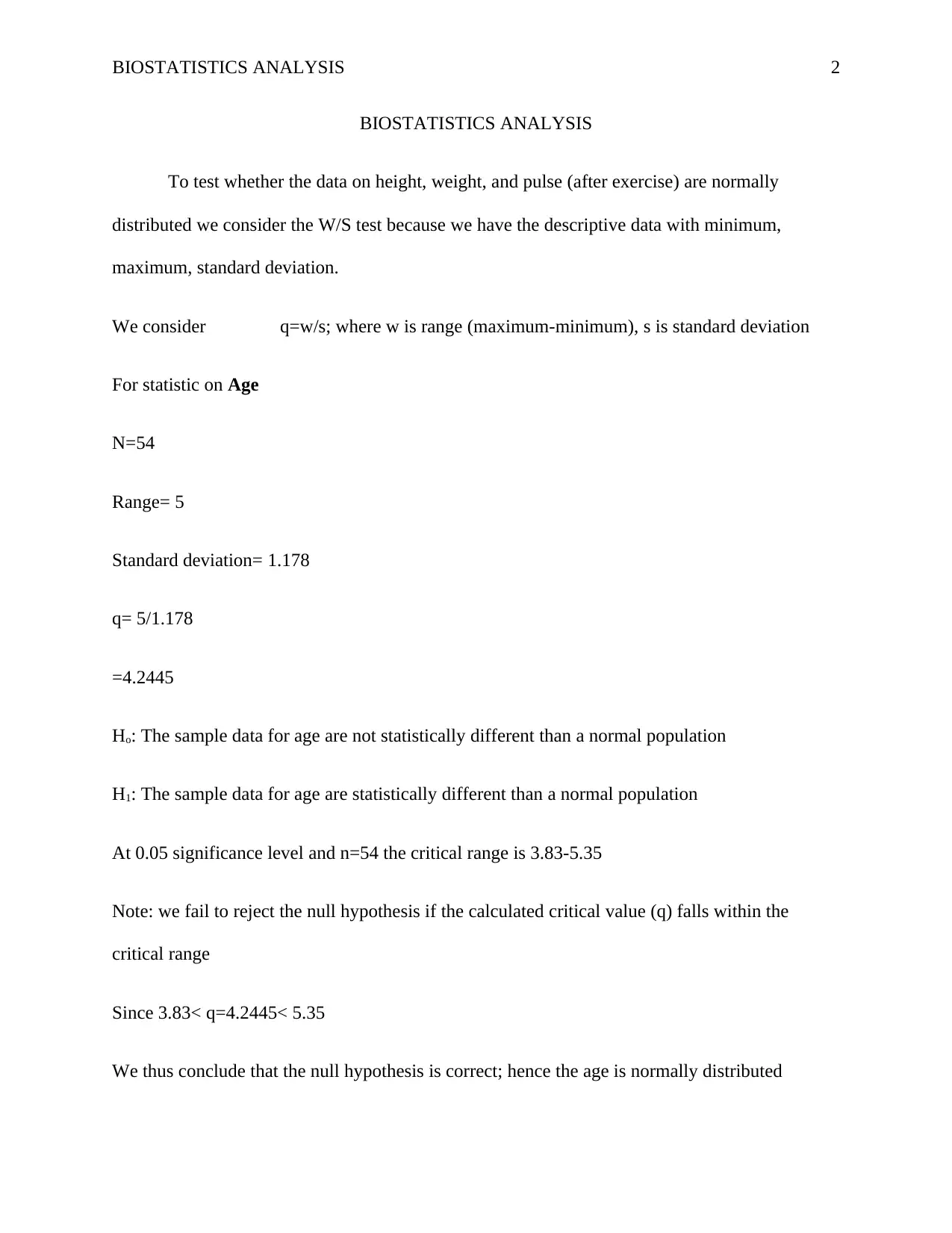
To test whether the data on height, weight, and pulse (after exercise) are normally
distributed we consider the W/S test because we have the descriptive data with minimum,
maximum, standard deviation.
We consider q=w/s; where w is range (maximum-minimum), s is standard deviation
For statistic on Age
N=54
Range= 5
Standard deviation= 1.178
q= 5/1.178
=4.2445
Ho: The sample data for age are not statistically different than a normal population
H1: The sample data for age are statistically different than a normal population
At 0.05 significance level and n=54 the critical range is 3.83-5.35
Note: we fail to reject the null hypothesis if the calculated critical value (q) falls within the
critical range
Since 3.83< q=4.2445< 5.35
We thus conclude that the null hypothesis is correct; hence the age is normally distributed

BIOSTATISTICS ANALYSIS 3
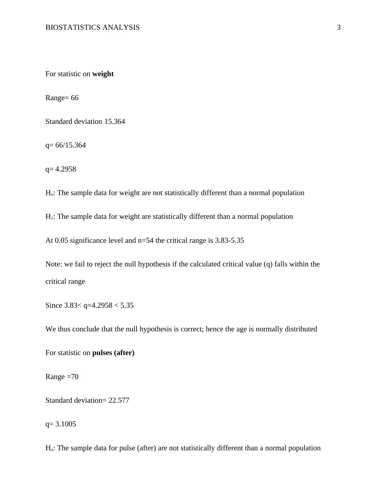
For statistic on weight
Range= 66
Standard deviation 15.364
q= 66/15.364
q= 4.2958
Ho: The sample data for weight are not statistically different than a normal population
H1: The sample data for weight are statistically different than a normal population
At 0.05 significance level and n=54 the critical range is 3.83-5.35
Note: we fail to reject the null hypothesis if the calculated critical value (q) falls within the
critical range
Since 3.83< q=4.2958 < 5.35
We thus conclude that the null hypothesis is correct; hence the age is normally distributed
For statistic on pulses (after)
Range =70
Standard deviation= 22.577
q= 3.1005
Ho: The sample data for pulse (after) are not statistically different than a normal population

BIOSTATISTICS ANALYSIS 4
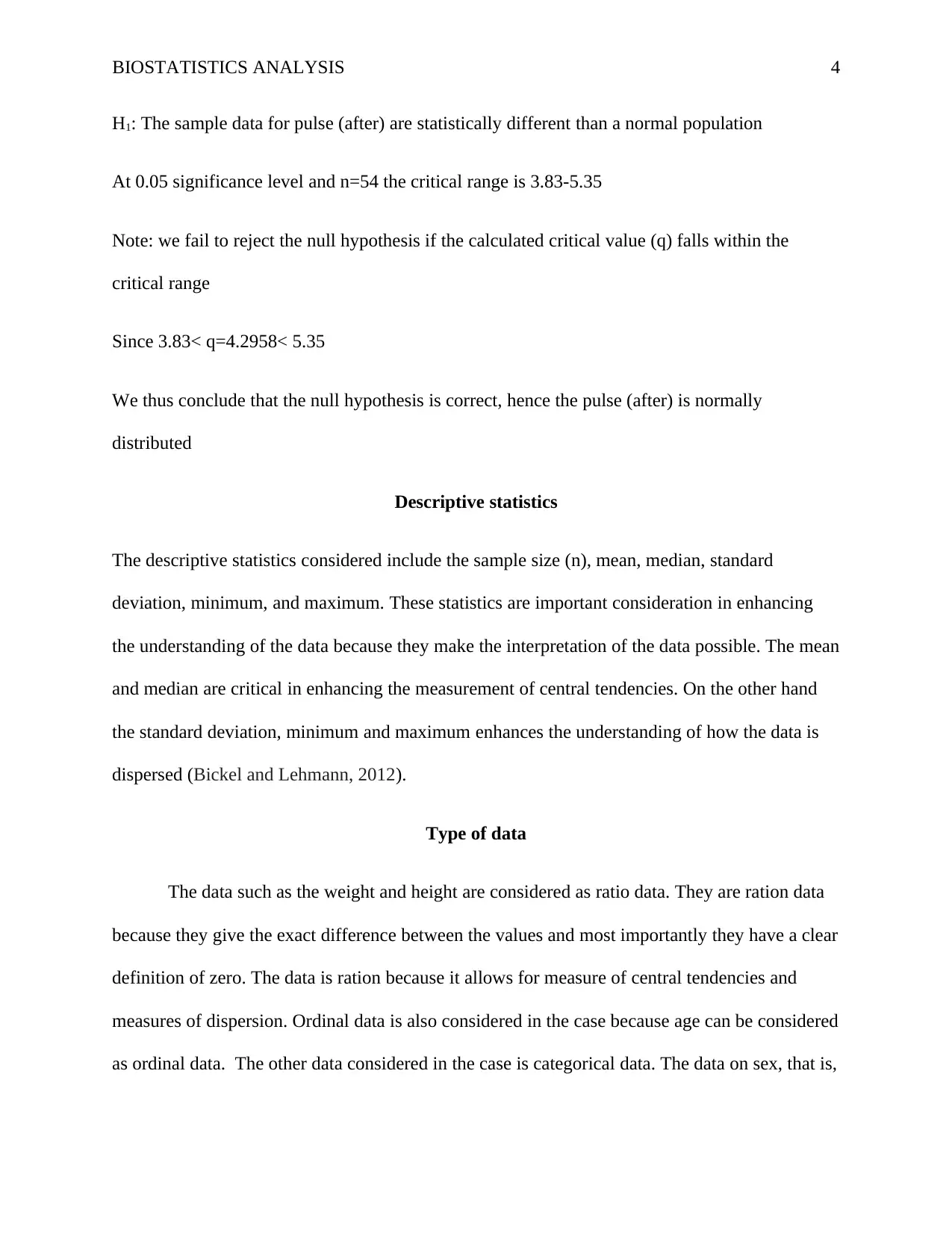
H1: The sample data for pulse (after) are statistically different than a normal population
At 0.05 significance level and n=54 the critical range is 3.83-5.35
Note: we fail to reject the null hypothesis if the calculated critical value (q) falls within the
critical range
Since 3.83< q=4.2958< 5.35
We thus conclude that the null hypothesis is correct, hence the pulse (after) is normally
distributed
Descriptive statistics
The descriptive statistics considered include the sample size (n), mean, median, standard
deviation, minimum, and maximum. These statistics are important consideration in enhancing
the understanding of the data because they make the interpretation of the data possible. The mean
and median are critical in enhancing the measurement of central tendencies. On the other hand
the standard deviation, minimum and maximum enhances the understanding of how the data is
dispersed (Bickel and Lehmann, 2012).
Type of data
The data such as the weight and height are considered as ratio data. They are ration data
because they give the exact difference between the values and most importantly they have a clear
definition of zero. The data is ration because it allows for measure of central tendencies and
measures of dispersion. Ordinal data is also considered in the case because age can be considered
as ordinal data. The other data considered in the case is categorical data. The data on sex, that is,

BIOSTATISTICS ANALYSIS 5
male and female can be considered as nominal data. Both continuous and discrete data are
utilized in the study. Height, weight and age are continuous while age and sex are discrete.
Parametric tests
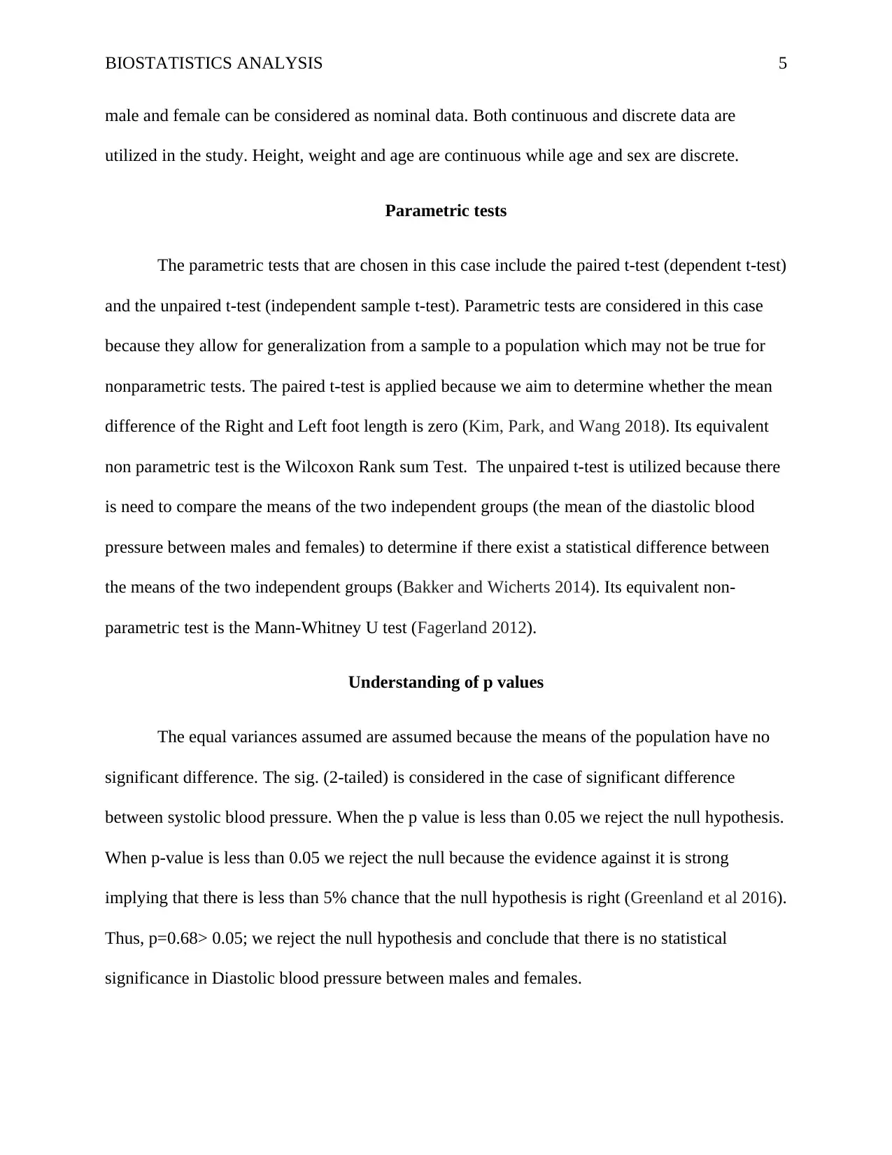
The parametric tests that are chosen in this case include the paired t-test (dependent t-test)
and the unpaired t-test (independent sample t-test). Parametric tests are considered in this case
because they allow for generalization from a sample to a population which may not be true for
nonparametric tests. The paired t-test is applied because we aim to determine whether the mean
difference of the Right and Left foot length is zero (Kim, Park, and Wang 2018). Its equivalent
non parametric test is the Wilcoxon Rank sum Test. The unpaired t-test is utilized because there
is need to compare the means of the two independent groups (the mean of the diastolic blood
pressure between males and females) to determine if there exist a statistical difference between
the means of the two independent groups (Bakker and Wicherts 2014). Its equivalent non-
parametric test is the Mann-Whitney U test (Fagerland 2012).
Understanding of p values
The equal variances assumed are assumed because the means of the population have no
significant difference. The sig. (2-tailed) is considered in the case of significant difference
between systolic blood pressure. When the p value is less than 0.05 we reject the null hypothesis.
When p-value is less than 0.05 we reject the null because the evidence against it is strong
implying that there is less than 5% chance that the null hypothesis is right (Greenland et al 2016).
Thus, p=0.68> 0.05; we reject the null hypothesis and conclude that there is no statistical
significance in Diastolic blood pressure between males and females.

BIOSTATISTICS ANALYSIS 6
Outcome of boxplot diagram
The male have only a single outlier while the females have six outliers hence showing
that data for the females is has more error than that of the males (Krzywinski and Altman 2014).
How and why distribution of male group has been influenced in the case
The distribution has been influenced by the fact that the chosen sample has the same weight
hence no many outliers. In the case the distribution of males is concentrated towards the mean
because of other external factors such as age. The age range of the sample is between 19 to 24
years. At the age group males are more likely to have the same weight.

BIOSTATISTICS ANALYSIS 7
References
Bakker, M. and Wicherts, J.M. (2014). Outlier removal, sum scores, and the inflation of the type
I error rate in independent samples t tests: The power of alternatives and
recommendations. Psychological methods, 19(3), p.409.
Bickel, P.J. and Lehmann, E.L. (2012). Descriptive statistics for nonparametric models I.
Introduction. In Selected Works of EL Lehmann (pp. 465-471). Springer, Boston, MA.
Fagerland, M.W. (2012). t-tests, non-parametric tests, and large studies—a paradox of statistical
practice?. BMC medical research methodology, 12(1), p.78.
Greenland, S., Senn, S.J., Rothman, K.J., Carlin, J.B., Poole, C., Goodman, S.N. and Altman,
D.G. (2016). Statistical tests, P values, confidence intervals, and power: a guide to
misinterpretations. European journal of epidemiology, 31(4), pp.337-350.
Kim, H., Park, C. and Wang, M. (2018). Paired t-test based on robustified statistics. 대대대대대대대 대대대대대대 대대대, pp.2347-2353.
Krzywinski, M. and Altman, N. (2014). Points of significance: visualizing samples with box
plots.