Biostatistics Assignment: Analysis of Income and Education Data

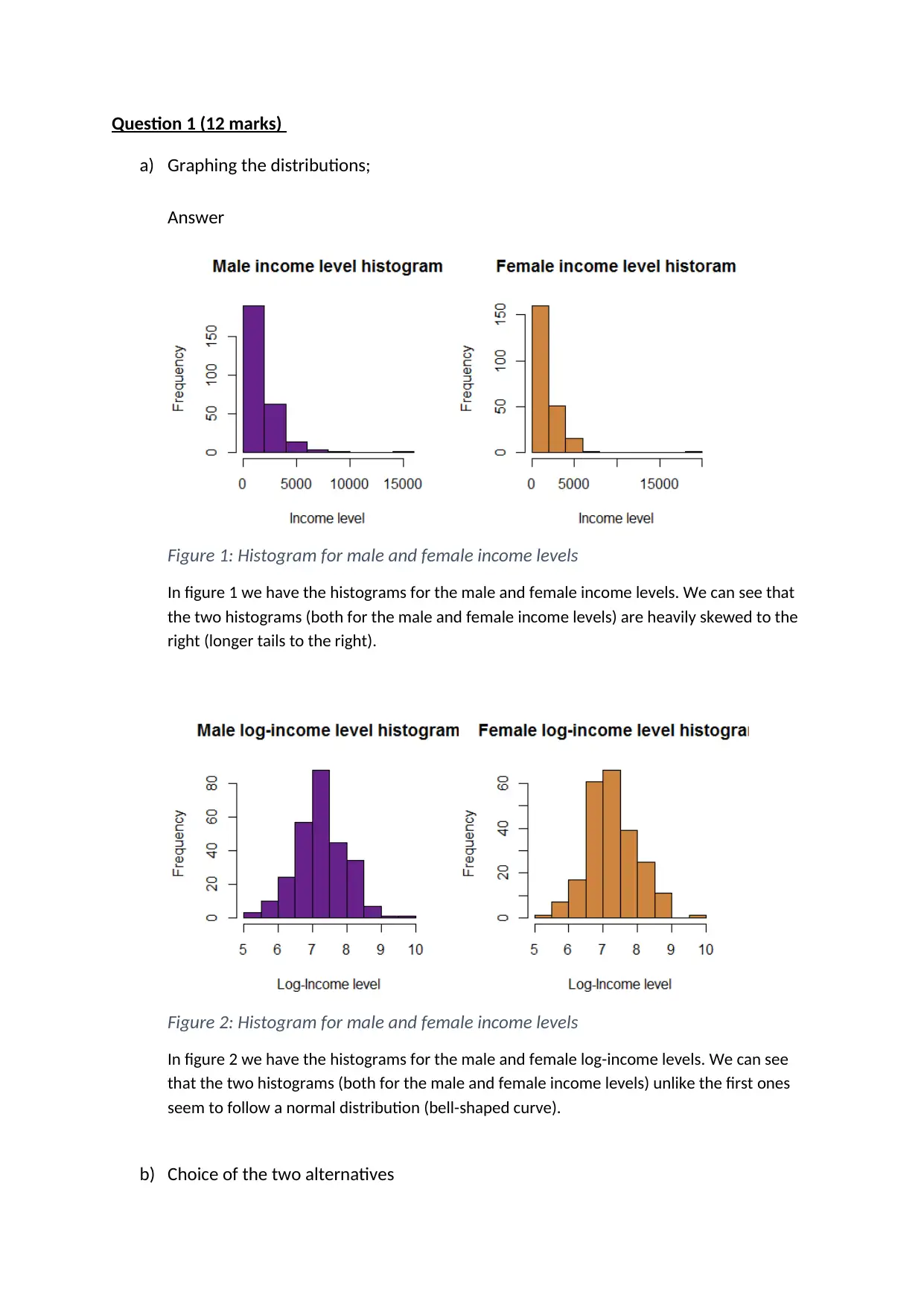
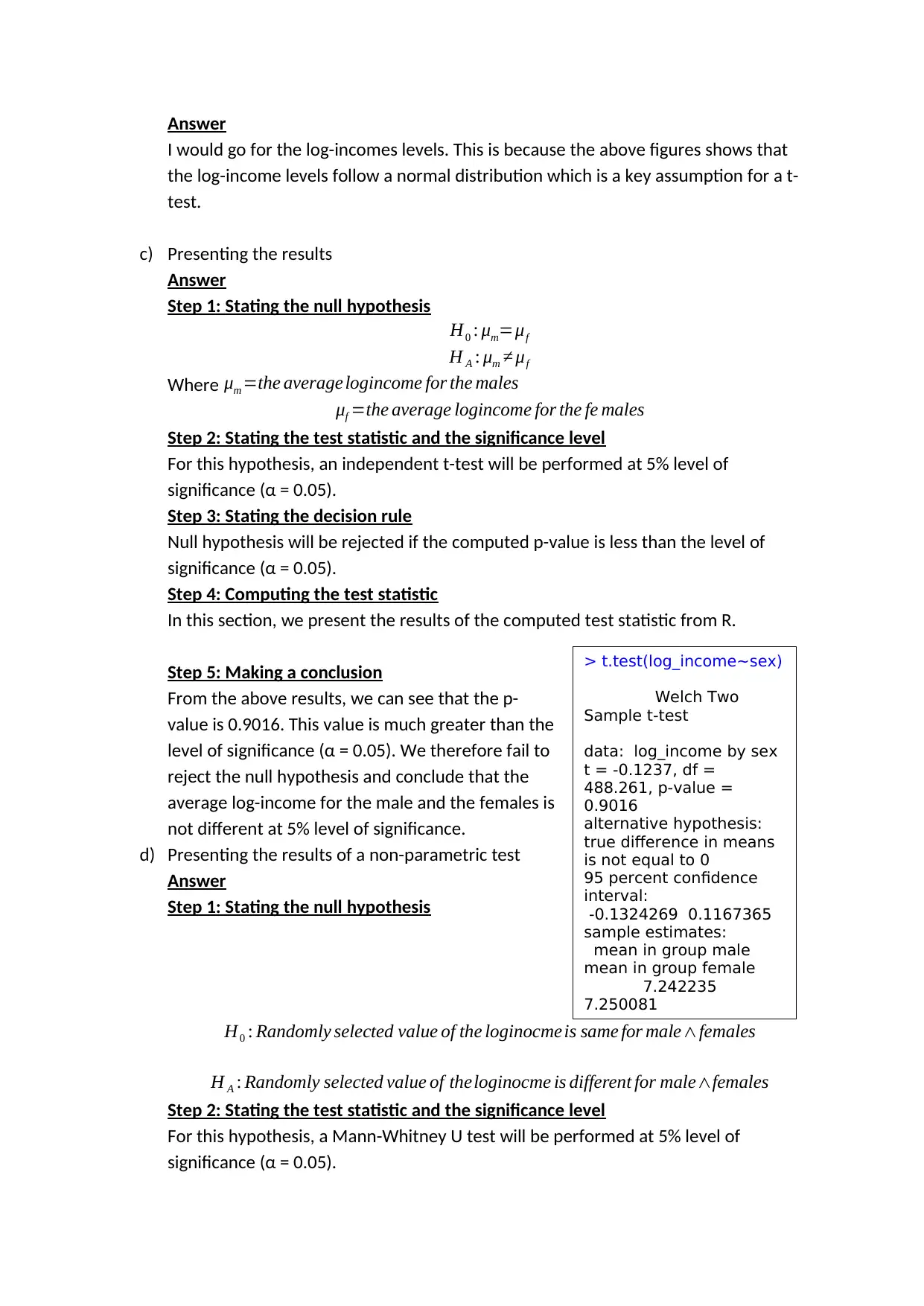
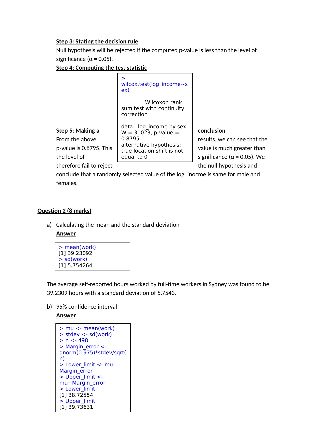
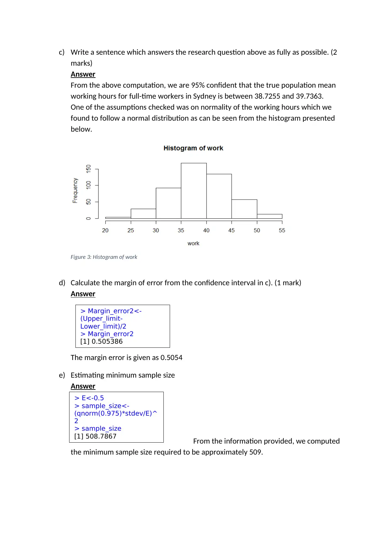
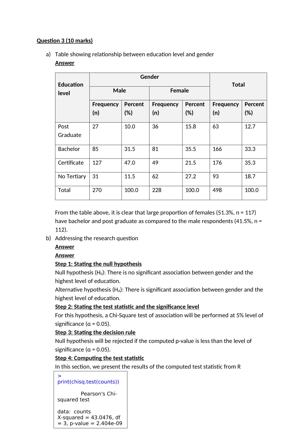
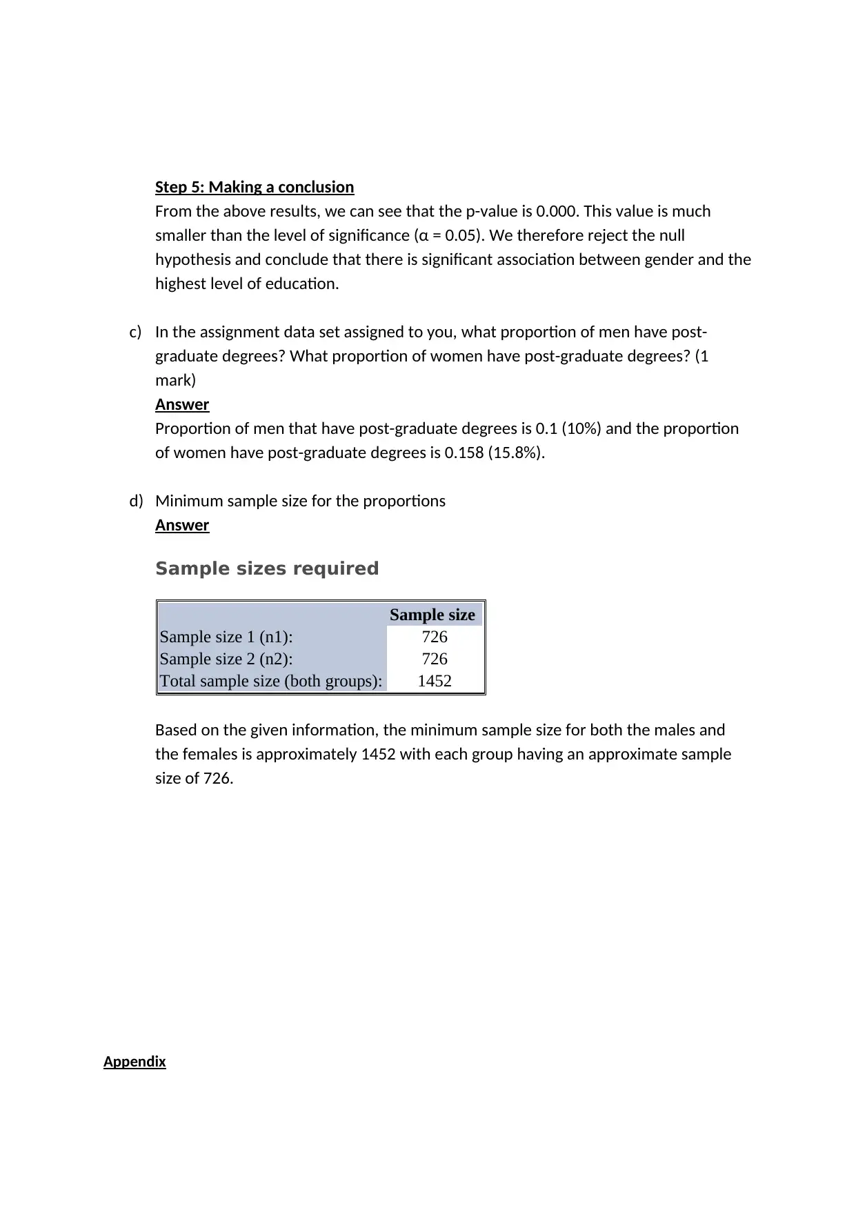
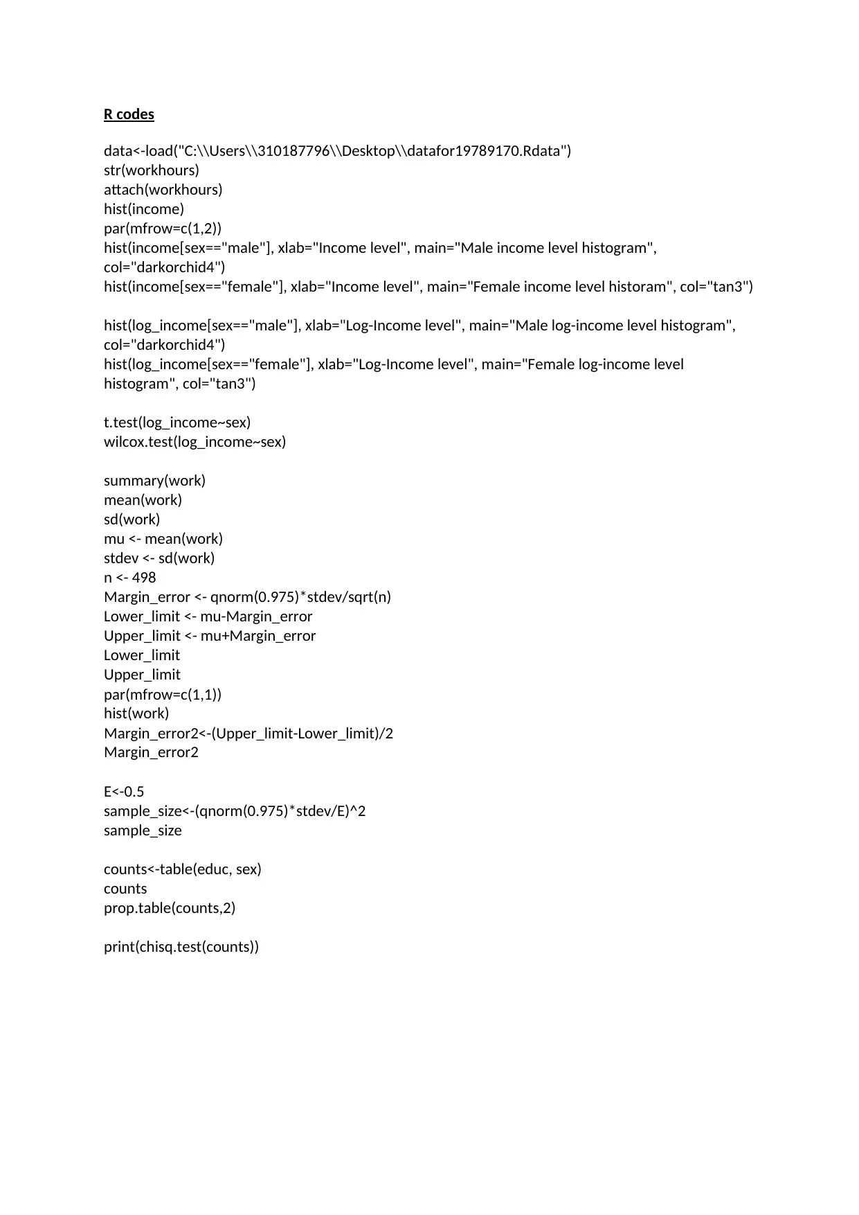
This biostatistics assignment analyzes a dataset related to income, education, and gender. The assignment includes several questions that require the application of statistical methods. Question 1 focuses on comparing income levels between males and females using t-tests and non-parametric tests, including the construction of histograms to assess data distribution. Question 2 involves calculating descriptive statistics, constructing confidence intervals, and determining the required sample size. Finally, Question 3 explores the relationship between education level and gender using a chi-square test, including the calculation of proportions and sample size requirements. The solution includes the presentation of results, hypothesis testing, and the interpretation of statistical outputs from R programming, along with the necessary R code used for the analysis. This assignment assesses the student's ability to apply statistical concepts to real-world data and draw meaningful conclusions.

Introduction to Bio-Statistics
Student Name:
Instructor Name:
Course Number:
6th May 2019

Question 1 (12 marks)
a) Graphing the distributions;
Answer
Figure 1: Histogram for male and female income levels
In figure 1 we have the histograms for the male and female income levels. We can see that
the two histograms (both for the male and female income levels) are heavily skewed to the
right (longer tails to the right).
Figure 2: Histogram for male and female income levels
In figure 2 we have the histograms for the male and female log-income levels. We can see
that the two histograms (both for the male and female income levels) unlike the first ones
seem to follow a normal distribution (bell-shaped curve).
b) Choice of the two alternatives

Answer
I would go for the log-incomes levels. This is because the above figures shows that
the log-income levels follow a normal distribution which is a key assumption for a t-
test.
c) Presenting the results
Answer
Step 1: Stating the null hypothesis
H0 : μm=μf
H A : μm ≠ μf
Where μm =the averagelogincome for the males
μf =the average logincome for the fe males
Step 2: Stating the test statistic and the significance level
For this hypothesis, an independent t-test will be performed at 5% level of
significance (α = 0.05).
Step 3: Stating the decision rule
Null hypothesis will be rejected if the computed p-value is less than the level of
significance (α = 0.05).
Step 4: Computing the test statistic
In this section, we present the results of the computed test statistic from R.
Step 5: Making a conclusion
From the above results, we can see that the p-
value is 0.9016. This value is much greater than the
level of significance (α = 0.05). We therefore fail to
reject the null hypothesis and conclude that the
average log-income for the male and the females is
not different at 5% level of significance.
d) Presenting the results of a non-parametric test
Answer
Step 1: Stating the null hypothesis
H0 : Randomly selected value of the loginocme is same for male∧females
H A : Randomly selected value of theloginocme is different for male∧females
Step 2: Stating the test statistic and the significance level
For this hypothesis, a Mann-Whitney U test will be performed at 5% level of
significance (α = 0.05).
> t.test(log_income~sex)
Welch Two
Sample t-test
data: log_income by sex
t = -0.1237, df =
488.261, p-value =
0.9016
alternative hypothesis:
true difference in means
is not equal to 0
95 percent confidence
interval:
-0.1324269 0.1167365
sample estimates:
mean in group male
mean in group female
7.242235
7.250081

Step 3: Stating the decision rule
Null hypothesis will be rejected if the computed p-value is less than the level of
significance (α = 0.05).
Step 4: Computing the test statistic
Step 5: Making a conclusion
From the above results, we can see that the
p-value is 0.8795. This value is much greater than
the level of significance (α = 0.05). We
therefore fail to reject the null hypothesis and
conclude that a randomly selected value of the log_inocme is same for male and
females.
Question 2 (8 marks)
a) Calculating the mean and the standard deviation
Answer
The average self-reported hours worked by full-time workers in Sydney was found to be
39.2309 hours with a standard deviation of 5.7543.
b) 95% confidence interval
Answer
>
wilcox.test(log_income~s
ex)
Wilcoxon rank
sum test with continuity
correction
data: log_income by sex
W = 31023, p-value =
0.8795
alternative hypothesis:
true location shift is not
equal to 0
> mean(work)
[1] 39.23092
> sd(work)
[1] 5.754264
> mu <- mean(work)
> stdev <- sd(work)
> n <- 498
> Margin_error <-
qnorm(0.975)*stdev/sqrt(
n)
> Lower_limit <- mu-
Margin_error
> Upper_limit <-
mu+Margin_error
> Lower_limit
[1] 38.72554
> Upper_limit
[1] 39.73631

c) Write a sentence which answers the research question above as fully as possible. (2
marks)
Answer
From the above computation, we are 95% confident that the true population mean
working hours for full-time workers in Sydney is between 38.7255 and 39.7363.
One of the assumptions checked was on normality of the working hours which we
found to follow a normal distribution as can be seen from the histogram presented
below.
Figure 3: Histogram of work
d) Calculate the margin of error from the confidence interval in c). (1 mark)
Answer
The margin error is given as 0.5054
e) Estimating minimum sample size
Answer
From the information provided, we computed
the minimum sample size required to be approximately 509.
> Margin_error2<-
(Upper_limit-
Lower_limit)/2
> Margin_error2
[1] 0.505386
> E<-0.5
> sample_size<-
(qnorm(0.975)*stdev/E)^
2
> sample_size
[1] 508.7867

Question 3 (10 marks)
a) Table showing relationship between education level and gender
Answer
Education
level
Gender
Total
Male Female
Frequency
(n)
Percent
(%)
Frequency
(n)
Percent
(%)
Frequency
(n)
Percent
(%)
Post
Graduate
27 10.0 36 15.8 63 12.7
Bachelor 85 31.5 81 35.5 166 33.3
Certificate 127 47.0 49 21.5 176 35.3
No Tertiary 31 11.5 62 27.2 93 18.7
Total 270 100.0 228 100.0 498 100.0
From the table above, it is clear that large proportion of females (51.3%, n = 117)
have bachelor and post graduate as compared to the male respondents (41.5%, n =
112).
b) Addressing the research question
Answer
Answer
Step 1: Stating the null hypothesis
Null hypothesis (H0): There is no significant association between gender and the
highest level of education.
Alternative hypothesis (HA): There is significant association between gender and the
highest level of education.
Step 2: Stating the test statistic and the significance level
For this hypothesis, a Chi-Square test of association will be performed at 5% level of
significance (α = 0.05).
Step 3: Stating the decision rule
Null hypothesis will be rejected if the computed p-value is less than the level of
significance (α = 0.05).
Step 4: Computing the test statistic
In this section, we present the results of the computed test statistic from R
>
print(chisq.test(counts))
Pearson's Chi-
squared test
data: counts
X-squared = 43.0476, df
= 3, p-value = 2.404e-09

Step 5: Making a conclusion
From the above results, we can see that the p-value is 0.000. This value is much
smaller than the level of significance (α = 0.05). We therefore reject the null
hypothesis and conclude that there is significant association between gender and the
highest level of education.
c) In the assignment data set assigned to you, what proportion of men have post-
graduate degrees? What proportion of women have post-graduate degrees? (1
mark)
Answer
Proportion of men that have post-graduate degrees is 0.1 (10%) and the proportion
of women have post-graduate degrees is 0.158 (15.8%).
d) Minimum sample size for the proportions
Answer
Sample sizes required
Sample size
Sample size 1 (n1): 726
Sample size 2 (n2): 726
Total sample size (both groups): 1452
Based on the given information, the minimum sample size for both the males and
the females is approximately 1452 with each group having an approximate sample
size of 726.
Appendix

R codes
data<-load("C:\\Users\\310187796\\Desktop\\datafor19789170.Rdata")
str(workhours)
attach(workhours)
hist(income)
par(mfrow=c(1,2))
hist(income[sex=="male"], xlab="Income level", main="Male income level histogram",
col="darkorchid4")
hist(income[sex=="female"], xlab="Income level", main="Female income level historam", col="tan3")
hist(log_income[sex=="male"], xlab="Log-Income level", main="Male log-income level histogram",
col="darkorchid4")
hist(log_income[sex=="female"], xlab="Log-Income level", main="Female log-income level
histogram", col="tan3")
t.test(log_income~sex)
wilcox.test(log_income~sex)
summary(work)
mean(work)
sd(work)
mu <- mean(work)
stdev <- sd(work)
n <- 498
Margin_error <- qnorm(0.975)*stdev/sqrt(n)
Lower_limit <- mu-Margin_error
Upper_limit <- mu+Margin_error
Lower_limit
Upper_limit
par(mfrow=c(1,1))
hist(work)
Margin_error2<-(Upper_limit-Lower_limit)/2
Margin_error2
E<-0.5
sample_size<-(qnorm(0.975)*stdev/E)^2
sample_size
counts<-table(educ, sex)
counts
prop.table(counts,2)
print(chisq.test(counts))