401077 Biostatistics Assignment 2: Income and Education Analysis

This biostatistics assignment analyzes a dataset of full-time workers in Sydney, addressing research questions related to income, working hours, and educational qualifications. The assignment utilizes R Commander for statistical analysis, including graphing distributions, conducting t-tests (both parametric and non-parametric), calculating confidence intervals, and determining required sample sizes. The analysis investigates whether there are income differences between genders, calculates average working hours with associated confidence intervals and margin of error, and examines the relationship between education level and gender using contingency tables and Chi-square tests. The assignment follows a 5-step method for hypothesis testing and provides detailed interpretations of the results, including the proportions of men and women with postgraduate degrees. R codes are also included in the appendix.

401077 Introduction to Biostatistics, Autumn 2019
Assignment 2
Statistics
Student Name:
Instructor Name:
Course Number:
22 April 2019

Question 1 (12 marks)
Research question: Does average self-reported weekly income differ between male and
female full-time workers in Sydney?
In the following analyses, use R Commander and the assignment data set assigned to you.
The variables you will use are ‘sex’ and ‘income’ and ‘log_income’. Each student will get
different answers as the data sets differ.
a) Using R Commander, graph the distributions of income for males and females
separately. Write a sentence describing the shape of these distributions. Repeat for
the logarithm transformed values of income (variable: log_income). (2 marks)
Answer
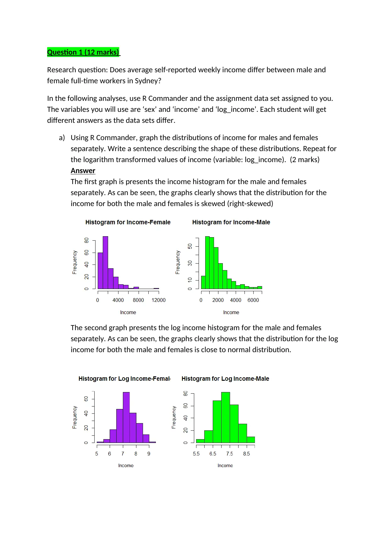
The first graph is presents the income histogram for the male and females
separately. As can be seen, the graphs clearly shows that the distribution for the
income for both the male and females is skewed (right-skewed)
The second graph presents the log income histogram for the male and females
separately. As can be seen, the graphs clearly shows that the distribution for the log
income for both the male and females is close to normal distribution.

b) The research question could be addressed by conducting either an independent
samples t-test on the difference in mean ‘income’ between genders or an
independent samples t-test on the difference in mean ‘log_income’ between
genders. Which of these two alternatives would you chose? Justify your choice. (2
marks)
Answer
I would chose an independent samples t-test on the difference in mean ‘log_income’
between genders. This is because one of the conditions for a t-test is that the data
should follow a normal distribution and from a) above, log_income was close to
normal distribution as compared to the income which was heavily skewed.
c) Using R Commander, implement the analysis you chose in b). Present your results
using the 5-step method. (4 marks)
Answer
Step1: Specifying the Hypothesis
We sought to test the following hypothesis
Null hypothesis (H0): There is no significant difference in the mean log_income
between the genders.
Alternative hypothesis (HA): There is significant difference in the mean log_income
between the genders.
Step 2: Set the Significance Level (a)
5% level of significance will be used to make a decision on whether to reject or to
accept the null hypothesis.
Step 3: Making a decision
Null hypothesis will be rejected if the computed p-value is less than the significance
level (α = 0.05)
Step 4: Computing the test statistic and the corresponding p-value
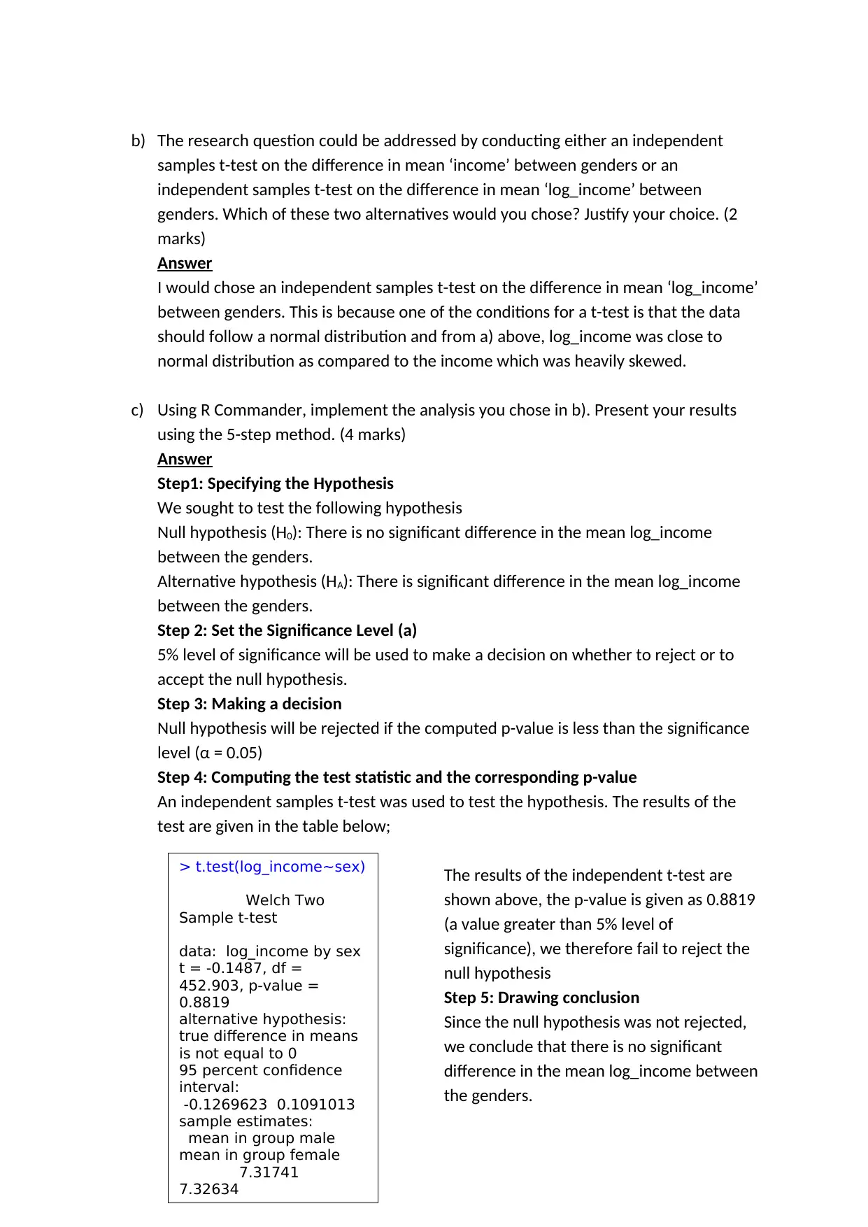
An independent samples t-test was used to test the hypothesis. The results of the
test are given in the table below;
The results of the independent t-test are
shown above, the p-value is given as 0.8819
(a value greater than 5% level of
significance), we therefore fail to reject the
null hypothesis
Step 5: Drawing conclusion
Since the null hypothesis was not rejected,
we conclude that there is no significant
difference in the mean log_income between
the genders.
> t.test(log_income~sex)
Welch Two
Sample t-test
data: log_income by sex
t = -0.1487, df =
452.903, p-value =
0.8819
alternative hypothesis:
true difference in means
is not equal to 0
95 percent confidence
interval:
-0.1269623 0.1091013
sample estimates:
mean in group male
mean in group female
7.31741
7.32634

d) The logarithm transformation changes the numeric values of the data but does not
change the order of data values. Therefore, a non-parametric hypothesis test (which
ranks the data) will give the same answer whether conducted on ‘income’ or ‘log-
income’. Complete an appropriate non-parametric test to address the research
question. Please use R Commander to do all calculations but present your answer
following the 5 step method. (4 marks)
Answer
Step1: Specifying the Hypothesis
We sought to test the following hypothesis
Null hypothesis (H0): The two samples (male and female) come from the same
population.
Alternative hypothesis (HA): The two samples (male and female) come from
significantly different populations.
Step 2: Set the Significance Level (a)
5% level of significance will be used to make a decision on whether to reject or to
accept the null hypothesis.
Step 3: Making a decision
Null hypothesis will be rejected if the computed p-value is less than the significance
level (α = 0.05)
Step 4: Computing the test statistic and the corresponding p-value
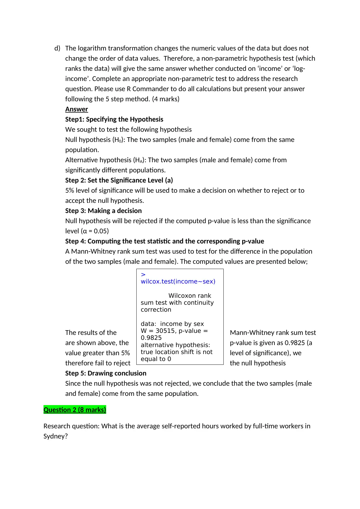
A Mann-Whitney rank sum test was used to test for the difference in the population
of the two samples (male and female). The computed values are presented below;
The results of the Mann-Whitney rank sum test
are shown above, the p-value is given as 0.9825 (a
value greater than 5% level of significance), we
therefore fail to reject the null hypothesis
Step 5: Drawing conclusion
Since the null hypothesis was not rejected, we conclude that the two samples (male
and female) come from the same population.
Question 2 (8 marks)
Research question: What is the average self-reported hours worked by full-time workers in
Sydney?
>
wilcox.test(income~sex)
Wilcoxon rank
sum test with continuity
correction
data: income by sex
W = 30515, p-value =
0.9825
alternative hypothesis:
true location shift is not
equal to 0

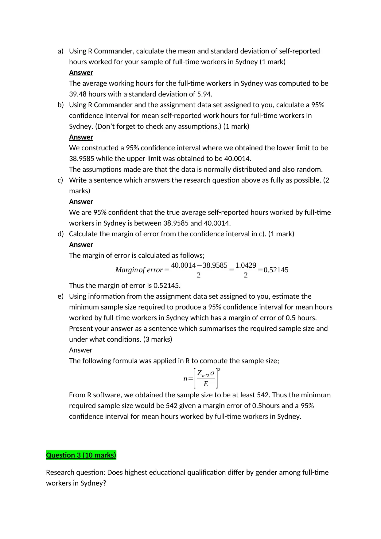
a) Using R Commander, calculate the mean and standard deviation of self-reported
hours worked for your sample of full-time workers in Sydney (1 mark)
Answer
The average working hours for the full-time workers in Sydney was computed to be
39.48 hours with a standard deviation of 5.94.
b) Using R Commander and the assignment data set assigned to you, calculate a 95%
confidence interval for mean self-reported work hours for full-time workers in
Sydney. (Don’t forget to check any assumptions.) (1 mark)
Answer
We constructed a 95% confidence interval where we obtained the lower limit to be
38.9585 while the upper limit was obtained to be 40.0014.
The assumptions made are that the data is normally distributed and also random.
c) Write a sentence which answers the research question above as fully as possible. (2
marks)
Answer
We are 95% confident that the true average self-reported hours worked by full-time
workers in Sydney is between 38.9585 and 40.0014.
d) Calculate the margin of error from the confidence interval in c). (1 mark)
Answer
The margin of error is calculated as follows;
Margin of error = 40.0014−38.9585
2 =1.0429
2 =0.52145
Thus the margin of error is 0.52145.
e) Using information from the assignment data set assigned to you, estimate the
minimum sample size required to produce a 95% confidence interval for mean hours
worked by full-time workers in Sydney which has a margin of error of 0.5 hours.
Present your answer as a sentence which summarises the required sample size and
under what conditions. (3 marks)
Answer
The following formula was applied in R to compute the sample size;
n=[ Zα /2 σ
E ]
2
From R software, we obtained the sample size to be at least 542. Thus the minimum
required sample size would be 542 given a margin error of 0.5hours and a 95%
confidence interval for mean hours worked by full-time workers in Sydney.
Question 3 (10 marks)
Research question: Does highest educational qualification differ by gender among full-time
workers in Sydney?

In the following analyses, use R Commander and the assignment data set assigned to you.
The variables you will use are ‘educ’ and ‘sex’. Each student will get different answers as the
data sets differ.
a) Investigate the relationship between highest education qualification obtained and
gender in the assignment data set assigned to you, using a two-way contingency
table. Include either row or column percentages and describe the observed
relationship in a sentence or two. Obtain the results using R Commander but then
type and label the table yourself with appropriate description and headings in your
answers. (2 marks)
Answer
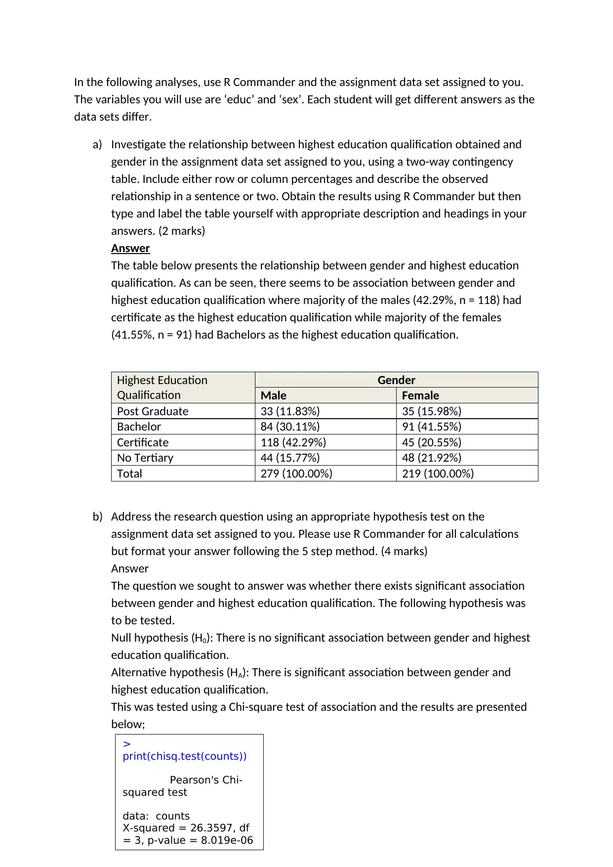
The table below presents the relationship between gender and highest education
qualification. As can be seen, there seems to be association between gender and
highest education qualification where majority of the males (42.29%, n = 118) had
certificate as the highest education qualification while majority of the females
(41.55%, n = 91) had Bachelors as the highest education qualification.
Highest Education
Qualification
Gender
Male Female
Post Graduate 33 (11.83%) 35 (15.98%)
Bachelor 84 (30.11%) 91 (41.55%)
Certificate 118 (42.29%) 45 (20.55%)
No Tertiary 44 (15.77%) 48 (21.92%)
Total 279 (100.00%) 219 (100.00%)
b) Address the research question using an appropriate hypothesis test on the
assignment data set assigned to you. Please use R Commander for all calculations
but format your answer following the 5 step method. (4 marks)
Answer
The question we sought to answer was whether there exists significant association
between gender and highest education qualification. The following hypothesis was
to be tested.
Null hypothesis (H0): There is no significant association between gender and highest
education qualification.
Alternative hypothesis (HA): There is significant association between gender and
highest education qualification.
This was tested using a Chi-square test of association and the results are presented
below;
>
print(chisq.test(counts))
Pearson's Chi-
squared test
data: counts
X-squared = 26.3597, df
= 3, p-value = 8.019e-06

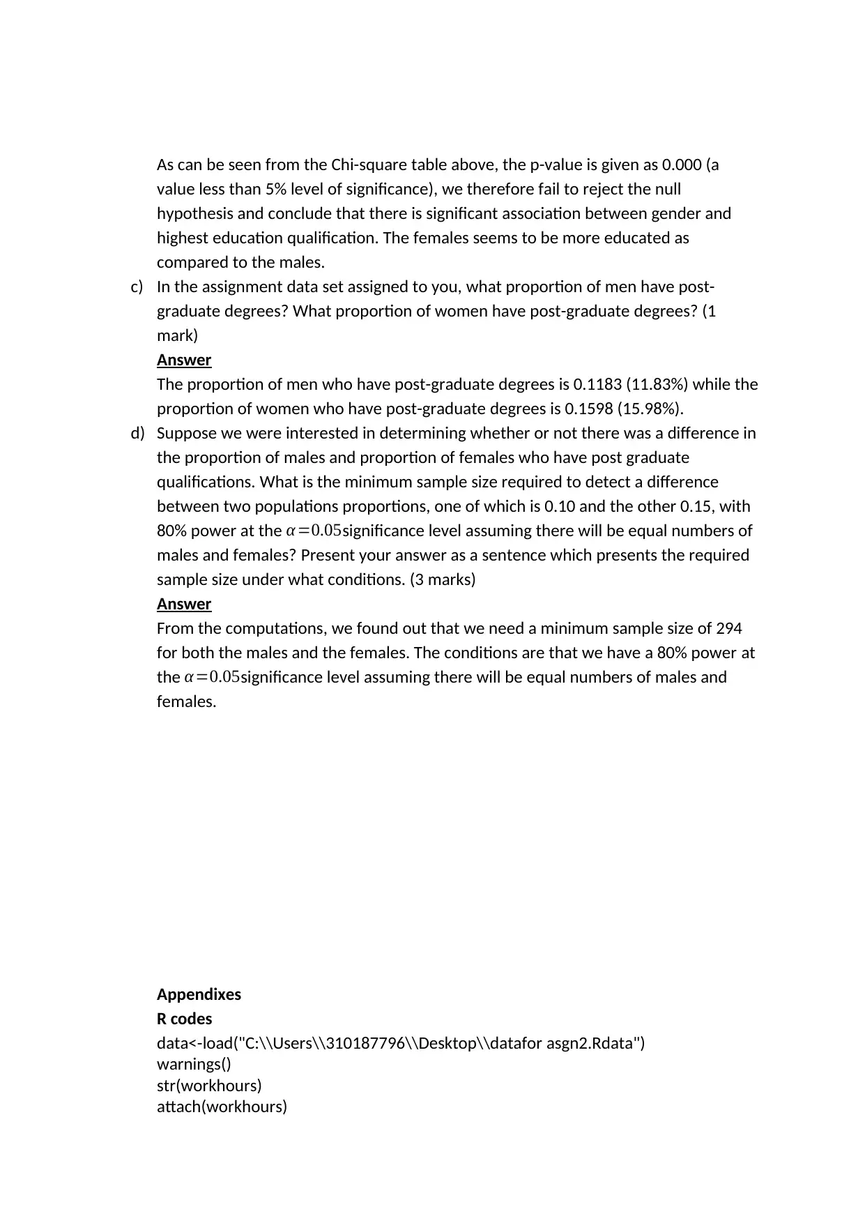
As can be seen from the Chi-square table above, the p-value is given as 0.000 (a
value less than 5% level of significance), we therefore fail to reject the null
hypothesis and conclude that there is significant association between gender and
highest education qualification. The females seems to be more educated as
compared to the males.
c) In the assignment data set assigned to you, what proportion of men have post-
graduate degrees? What proportion of women have post-graduate degrees? (1
mark)
Answer
The proportion of men who have post-graduate degrees is 0.1183 (11.83%) while the
proportion of women who have post-graduate degrees is 0.1598 (15.98%).
d) Suppose we were interested in determining whether or not there was a difference in
the proportion of males and proportion of females who have post graduate
qualifications. What is the minimum sample size required to detect a difference
between two populations proportions, one of which is 0.10 and the other 0.15, with
80% power at the α =0.05significance level assuming there will be equal numbers of
males and females? Present your answer as a sentence which presents the required
sample size under what conditions. (3 marks)
Answer
From the computations, we found out that we need a minimum sample size of 294
for both the males and the females. The conditions are that we have a 80% power at
the α=0.05significance level assuming there will be equal numbers of males and
females.
Appendixes
R codes
data<-load("C:\\Users\\310187796\\Desktop\\datafor asgn2.Rdata")
warnings()
str(workhours)
attach(workhours)

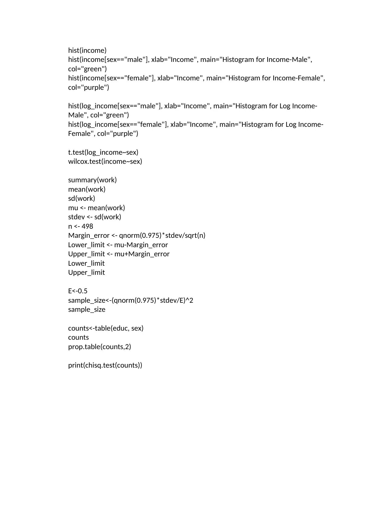
hist(income)
hist(income[sex=="male"], xlab="Income", main="Histogram for Income-Male",
col="green")
hist(income[sex=="female"], xlab="Income", main="Histogram for Income-Female",
col="purple")
hist(log_income[sex=="male"], xlab="Income", main="Histogram for Log Income-
Male", col="green")
hist(log_income[sex=="female"], xlab="Income", main="Histogram for Log Income-
Female", col="purple")
t.test(log_income~sex)
wilcox.test(income~sex)
summary(work)
mean(work)
sd(work)
mu <- mean(work)
stdev <- sd(work)
n <- 498
Margin_error <- qnorm(0.975)*stdev/sqrt(n)
Lower_limit <- mu-Margin_error
Upper_limit <- mu+Margin_error
Lower_limit
Upper_limit
E<-0.5
sample_size<-(qnorm(0.975)*stdev/E)^2
sample_size
counts<-table(educ, sex)
counts
prop.table(counts,2)
print(chisq.test(counts))