Biostatistical Methods PHC6052: Course Project Step 4 Final Discussion

This assignment presents solutions to the final discussion questions for Course Project Step 4 in a Biostatistics course, focusing on the application of statistical inference in three cases: QQ, CC, and CQ. The analysis covers descriptive summaries of explanatory and response variables, correlation and linear regression analysis, and chi-square tests. Specific questions address the distribution of variables, the appropriateness of statistical methods, interpretation of correlation coefficients and regression equations, and the validity of model assumptions based on residual analysis. The assignment also examines the association between categorized variables using chi-square tests and discusses the distribution of binary responses within multi-level explanatory variables. The solutions are based on the results obtained from a previous step (Step 3) and emphasize the importance of understanding the conditions for using each statistical test.

Course Project Step 4 - Final Discussion Questions on Analyses Conducted
This is a preview of the published version of the quiz
Quiz Instructions
Use ONLY your final results for STEP 3 to answer the questions on this assignment.
BONUS for EARLY SUBMISSION = 1 point for each day prior to the deadline starting November
29th!! (Nov 29th = 5 points, 30th = 4 points, ... , Dec 3rd = 1 point)
Purpose: Apply statistical inference in the three cases covered in this course (QQ, CC, CQ) correctly
and also to see how we can approach the same question using different types of variables and
thus different methods.
We are picking apart the overall analyses into many sub-questions. Please carefully review all
questions related to each part from the STEP 3 analysis before beginning those questions and be
sure to address only the current question in each answer.
No remediation will be offered for this final assessment.
Note: Fill-in-the-blank questions will be marked incorrect in auto grading and must be hand graded
based upon your STEP 3 results.
Question 1
FROM STEP 3 PART 1: Descriptive Summary of EXPLANATORY variable
Provide a brief discussion of the distribution of your EXPLANATORY variable using as much of the
relevant information in STEP 3 Questions 1-4 as possible (and yet remain as concise as possible). Be
sure to include information from each question in STEP 3 Part 1.
The explanatory variable is also known as independent variable, in this study, the explanatory
variable is “Waist (Inches)”. The total number of variables for waist are 400 with mean 37.92 inches,
median 37 inches and standard deviation 5.72 inches. The shape of the distribution is slightly
skewed to the right as mean is greater than median. The histogram for waist indicates that the data
is slightly skewed at the right as the most of the frequencies for waist is obtained for 37 inches. The
boxplot indicates that the data for waist contains two outliers and the Q-Q plot indicates that data
for waist is light tailed.
Question 2
FROM STEP 3 PART 2: Descriptive Summary of RESPONSE variable
Provide a brief discussion of the distribution of your RESPONSE variable using as much of the
relevant information in STEP 3 Questions 5-8 as possible (and yet remain as concise as possible). Be
sure to include information from each question in STEP 3 Part 2.
The response variable is also known as dependent variable, in this study, the explanatory variable is
“Weight (Pounds)”. The total number of variables for waist are 400 with mean 177.76 pounds,
median 173 pounds and standard deviation 40.37 pounds. The shape of the distribution is slightly
skewed to the right as mean is greater than median. The histogram for weight indicates that the
data is slightly skewed at the right as the most of the frequencies for weight is obtained for 180
Pounds. The boxplot indicates that the data for weight contains outliers and the Q-Q plot indicates
that data for weight is light tailed.
Question 3
FROM STEP 3 PART 3: Case QQ - Using the two quantitative variables to investigate relationship
 Based upon the scatterplot between your quantitative response and your quantitative
explanatory variable, do you feel Pearson’s correlation and linear
regression are reasonable analyses to use?
 Explain clearly what you see in the scatterplot to justify your answer.
Your answer should be 1-3 sentences.
The correlation is statistically significant because the P-value is (0.0001) is less than the level of
significance (Say 0.05). Hence, it can say that the Pearson’s correlation and linear regression are
reasonable to use.
The scatterplot between the weight and waist indicates that as the waist increases strongly the
weight also increases strongly. The correlation between the variables weight and weight is 0.8498
which is near to one and indicates a strong positive linear relationship between the variables.
Question 4
Note: Answers to this question will be automatically marked incorrect. We will need to review them
manually to determine if they are correct based upon your STEP 3 output.
Answer this question regardless of any decisions regarding the conditions for using this method.
FROM STEP 3 PART 3: Case QQ - Using the two quantitative variables to investigate relationship
Provide the exact values given by the software for the items requested below.
 The value of Pearson’s correlation coefficient: 0.84985
 The associated two-sided p-value: 0.000 (Less than 0.0001)
Question 5
FROM STEP 3 PART 3: Case QQ - Using the two quantitative variables to investigate relationship
 Based upon the value of Pearson’s correlation coefficient, what can you say about
the strength and direction of “the best line” through your data?
 Explain how this coincides with what is seen in your scatterplot.
Your answer should be 1-3 sentences.
A correlation of 0.8498 indicates that the best line through the data has a strong increasing
relationship. The scatterplot shows a linear relationship that is strong and increasing. The
correlation provides a good summary of the strength and direction of the relationship for this data.

Question 6
Note: Answers to this question will be automatically marked incorrect. We will need to review them
manually to determine if they are correct based upon your STEP 3 output.
Answer this question regardless of any decisions regarding the conditions for using this method.
FROM STEP 3 PART 3: Case QQ - Using the two quantitative variables to investigate relationship
 Using the exact values given by the software needed, write the regression equation for
“the best line” through your data:
Y-hat = -49.579 + 5.99 (Waist)
Question 7
Note: Answers to this question will be automatically marked incorrect. We will need to review them
manually to determine if they are correct based upon your STEP 3 output.
Answer this question regardless of any decisions regarding the conditions for using this method.
FROM STEP 3 PART 3: Case QQ - Using the two quantitative variables to investigate relationship
Provide the exact values given by the software as needed to interpret the coefficient of
determination, R-square, in context:
 Approximately 72.23 percent of the variation in weight can be explained by this simple linear
regression model using waist.
Question 8
Note: Answers to this question will be automatically marked incorrect. We will need to review them
manually to determine if they are correct based upon your STEP 3 output.
Answer this question regardless of any decisions regarding the conditions for using this method.
FROM STEP 3 PART 3: Case QQ - Using the two quantitative variables to investigate relationship
Provide the exact values given by the software as needed to interpret the slope of “the best line”
through your data in context.
Interpret this value about the “best line” regardless of whether this “best line” is a good model for
your data.
 For each 1-unit increase in waist the weight is expected to increase by 5.99.
Question 9
FROM STEP 3 PART 3: Case QQ - Using the two quantitative variables to investigate relationship
 Based upon the histogram and PP-plot of the residuals, explain whether or not you feel the
distribution of the residuals is reasonably normal.
 Explain clearly what you see in the plots to justify your answer.
Your answer should be 1-3 sentences.
The distributions of residuals are reasonably normal, because the histogram of residuals is not
skewed and the PP-plot of residuals indicates that all the residuals are scattered over the central line
0.
The PP-Plot indicates that the residuals are scattered above and below the central line 0, thus it can
say that residuals are unbiased and homoscedastic.
Question 10
FROM STEP 3 PART 3: Case QQ - Using the two quantitative variables to investigate relationship
 Based upon the scatterplot of the residuals vs. the predicted values, explain whether or not you
feel the error term for the regression model has constant variance.
 Explain clearly what you see in this scatterplot to justify your answer.
Your answer should be 1-3 sentences.
The QQ-plot of residuals indicates that all the residuals are within confidence limits.
The QQ-Plot indicates that most of the residuals are lying on the normal line and rest belongs within
confidence limits.
Question 11
FROM STEP 3 PART 3: Case QQ - Using the two quantitative variables to investigate relationship
Based upon whether or not you feel linear regression is appropriate, answer one of the following:
 If linear regression is appropriate, state the p-value for the slope and provide the conclusion to
the hypothesis test associated with this p-value in context.
 If linear regression is not appropriate, summarize the reasons you have discovered very briefly.
You do not need to repeat any previous explanations just state the issues involved which make you
feel linear regression is not appropriate for your data.
Your answer should be 1-2 sentences.
The P-value for slope is approximately 0.000. Now comparing the P-value with the level of
significance (Say 0.05), P-value is less than 0.05, so the null hypothesis is rejected and it is concluded
that the slope is not equal to zero. Hence, linear regression is appropriate.

Question 12
Question 12
FROM STEP 3 PART 4: Case CC – Using categorized versions of response and explanatory to
investigate relationship
 Are the conditions for using the appropriate chi-square test satisfied for all combinations
investigated in Part 4 of STEP3?
 Why or why not? Be sure to specify very clearly any combinations for which the conditions
are not satisfied.
The chi-square test will be used if expected frequency is greater than or equal to 5. According to
the provided outputs, the expected frequency for BINARY EXPLANATORY variable and BINARY
RESPONSE, MULTI-LEVEL EXPLANATORY variable and MULTI-LEVEL RESPONSE variable, BINARY
EXPLANATORY variable and MULTI-LEVEL RESPONSE variable and MULTI-LEVEL EXPLANATORY
variable and BINARY RESPONSE variable are greater than 5. Thus, the conditions for using chi-
square test is satisfied for all the combinations.
Question 13
Note: Answers to this question will be automatically marked incorrect. We will need to review
them manually to determine if they are correct based upon your STEP 3 output.
FROM STEP 3 PART 4: Case CC – Using categorized versions of response and explanatory to
investigate relationship
 For each combination below provide the name of the appropriate chi-square statistic used,
it’s associated p-value, and fill in the appropriate information to complete the conclusion in
context for each test.
 Answer this question completely regardless of your answer to the previous question
regarding the conditions for using these tests.
STEP 3 Q12: BINARY EXPLANATORY variable and BINARY RESPONSE variable
 Name of Test Statistic: Chi-Square test.
 P-Value: <0.0001
 There is not enough evidence that an association exists between BINARY EXPLANATORY
variable and BINARY RESPONSE variable.
STEP 3 Q13: MULTI-LEVEL EXPLANATORY variable and MULTI-LEVEL RESPONSE variable
Name of Test Statistic: Chi-Square test.
 P-Value: <0.0001
 There is not enough evidence that an association exists between MULTI-LEVEL EXPLANATORY
variable and MULTI-LEVEL RESPONSE variable.
.

STEP 3 Q14: BINARY EXPLANATORY variable and MULTI-LEVEL RESPONSE variable
 Name of Test Statistic: Chi-Square test.
 P-Value: <0.0001
 There is not enough evidence that an association exists between BINARY EXPLANATORY variable
and MULTI-LEVEL RESPONSE variable.
STEP 3 Q15: MULTI-LEVEL EXPLANATORY variable and BINARY RESPONSE variable
 Name of Test Statistic: Chi-Square test.
 P-Value: <0.0001
 There is not enough evidence that an association exists between MULTI-LEVEL EXPLANATORY
variable and BINARY RESPONSE variable.
Question 14
FROM STEP 3 PART 4: Case CC – Using categorized versions of response and explanatory to
investigate relationship
For the results produced in STEP 3 Question 15, involving the multi-level explanatory variable and
the binary response variable:
 Provide a discussion of the distribution of your BINARY RESPONSE within the levels of the
MULTI-LEVEL EXPLANATORY variable.
Note: This is similar to the questions on the assignments which related to comparing conditional
percentages in Case CC.
The chi-square value for the test is 194.06, and the corresponding P-value is less than 0.001, so the
null hypothesis of test gets rejected and it can conclude that there is no associa tion exists between
MULTI-LEVEL EXPLANATORY variable and BINARY RESPONSE variable.
Question 15
FROM STEP 3 PART 5: Case CQ – Using your quantitative response variable and the binary version
of your explanatory variable
 Are the conditions for using the two-sample t-test for independent samples satisfied?
 Why or why not?
 Note: If you feel you need additional output to answer this question, you do not need to obtain
it, instead specify what you would obtain and explain what you would be looking for.

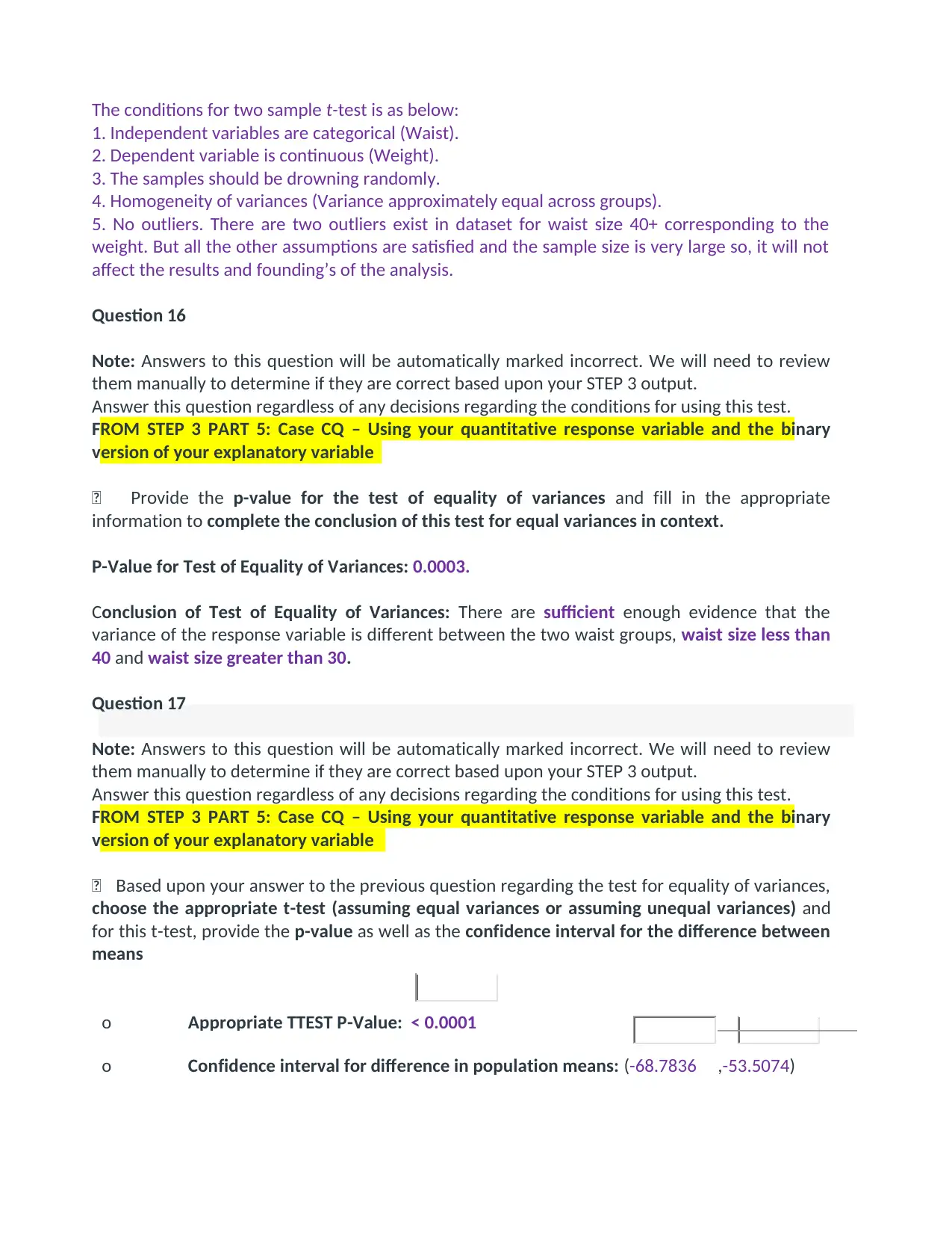
The conditions for two sample t-test is as below:
1. Independent variables are categorical (Waist).
2. Dependent variable is continuous (Weight).
3. The samples should be drowning randomly.
4. Homogeneity of variances (Variance approximately equal across groups).
5. No outliers. There are two outliers exist in dataset for waist size 40+ corresponding to the
weight. But all the other assumptions are satisfied and the sample size is very large so, it will not
affect the results and founding’s of the analysis.
Question 16
Note: Answers to this question will be automatically marked incorrect. We will need to review
them manually to determine if they are correct based upon your STEP 3 output.
Answer this question regardless of any decisions regarding the conditions for using this test.
FROM STEP 3 PART 5: Case CQ – Using your quantitative response variable and the binary
version of your explanatory variable
 Provide the p-value for the test of equality of variances and fill in the appropriate
information to complete the conclusion of this test for equal variances in context.
P-Value for Test of Equality of Variances: 0.0003.
Conclusion of Test of Equality of Variances: There are sufficient enough evidence that the
variance of the response variable is different between the two waist groups, waist size less than
40 and waist size greater than 30.
Question 17
Note: Answers to this question will be automatically marked incorrect. We will need to review
them manually to determine if they are correct based upon your STEP 3 output.
Answer this question regardless of any decisions regarding the conditions for using this test.
FROM STEP 3 PART 5: Case CQ – Using your quantitative response variable and the binary
version of your explanatory variable
 Based upon your answer to the previous question regarding the test for equality of variances,
choose the appropriate t-test (assuming equal variances or assuming unequal variances) and
for this t-test, provide the p-value as well as the confidence interval for the difference between
means
o Appropriate TTEST P-Value: < 0.0001
o Confidence interval for difference in population means: (-68.7836 ,-53.5074)

Question 18
Answer this question regardless of any decisions regarding the conditions for using this test.
FROM STEP 3 PART 5: Case CQ – Using your quantitative response variable and the binary
version of your explanatory variable
Using the results from the previous question:
 Provide one sentence stating the conclusion in context for the two-sample t-test.
 Provide one sentence with the interpretation of the confidence interval for the difference
between the two population means. If the t-test is statistically significant, be sure your
interpretation includes which group mean is larger or smaller than the other and by how much.
According to the 2 sample t-test output the t-value is -16.77, p-value is 0.0001, now compare the
P-value with the level of significance (Say 0.05), the P-value (0.0001) is less than level of
significance 0.05. Hence, null hypothesis gets rejected and it can be concluded that there is
statistically significant difference in the mean of waist size less than 40 and waist size greater than
30 corresponding to the weight. The mean of waist size greater than 40 is larger than the mean
of the waist size less than 40 by 60.7 inches.
Question 19
Consider the conclusion provided to the test in the previous question.
 Which type of error could you have made with your conclusion to the two sample t-test?
 What would this error imply in the context of your data?
Your answer should be 1-3 sentences.
Reject the null hypothesis when it is true will make type I error, if we reject the null hypothesis
that there is no difference between the means of waist size greater than 40 and the mean of the
waist size less than 40 when it is true then type I error will happen.
Accept the null hypothesis when it is false will make type II error, if we does not reject the null
hypothesis that there is no difference between the means of waist size greater than 40 and the
mean of the waist size less than 40 when it is false then type II error will happen.
Question 20
FROM STEP 3 PART 6: Case CQ – Using your quantitative response variable and the multi-level
version of your explanatory
 Are the conditions for using the one-way ANOVA satisfied?

 Why or why not?
 If you feel you need additional output to answer this question, you do not need to obtain it,
instead specify what you would obtain and explain what you would be looking for.
Length may vary; keep your answer as brief as possible while addressing the question.
1. Dependent variable (weight) should be measured at the continuous level.
2. Independent variables (Multilevel waist) should consist of two or more categorical,
independent groups.
3. The observations should be independent which means that there is no relationship between
the observations in each group or between the groups.
4. There should be no significant outliers. The Boxplot for the multilevel independent variable
corresponding to the response variable weight, not indicates strong outliers.
5. Dependent variable should be approximately normally distributed for each combination of the
groups of the independent variables.
6. There needs to be homogeneity of variances for each combination of the groups of the two
independent variables. So the Levene’s test for homogeneity of variances will useful.
Question 21
Note: Answers to this question will be automatically marked incorrect. We will need to review
them manually to determine if they are correct based upon your STEP 3 output.
Answer this question regardless of any decisions regarding the conditions for using this test.
FROM STEP 3 PART 6: Case CQ – Using your quantitative response variable and the multi-level
version of your explanatory
 Provide the p-value of the one-way ANOVA test and fill in the appropriate information to
complete the conclusion in context.
P-Value for One-Way ANOVA: <0.0001
Conclusion: There is significant enough evidence that mean weight corresponding to the four
multilevel explanatory variables are different.
Question 22.
Consider the conclusion provided to the test in the previous question.
 Which type of error could you have made with your conclusion to this ANOVA test?
 Explain what this error would imply in the context of your data. Your answer should be 1-3
sentences.
Accept the null hypothesis when it is false will make type II error, if we does not reject the null
hypothesis that there is no difference between the means of four multilevel when it is false then
type II error will happen.

Question 23.
OVERALL SUMMARY
 Explain which appropriate and valid method you prefer as your primary method to analyze
this data and why.
Length may vary; keep your answer as brief as possible while addressing the question.
Both the variable weight and waist are categorical, so the chi-square test will be used for the
analysis. This test will indicate the relationship between the binary and multilevel variables
corresponding to the weight and waist.
The multilevel binary logistic regression or binary logistic regression can be used for forecasting
of weight.
Question 24
Consider the tasks involved in the entire course project (STEPS 1-4).
At the beginning of the semester what percent (0 to 100) of these concepts and ideas were you
already familiar with?
You may also provide any explanations or other comments you wish to share.
Please do by yourself.