Introduction to Biostatistics Assignment: Analysis and Modeling

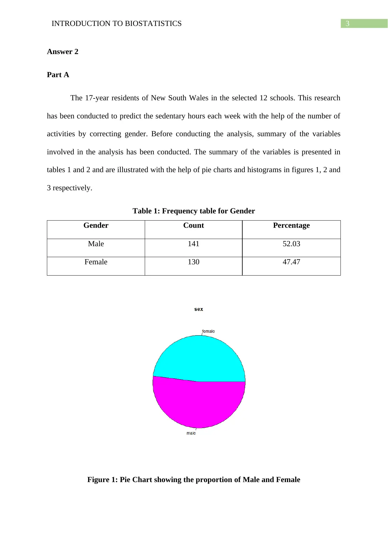
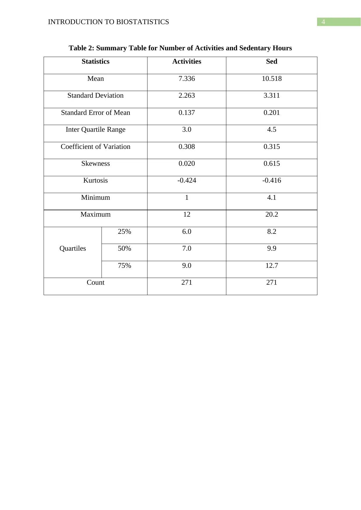
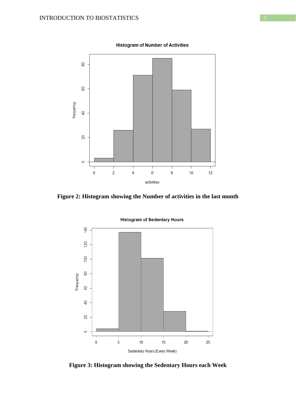
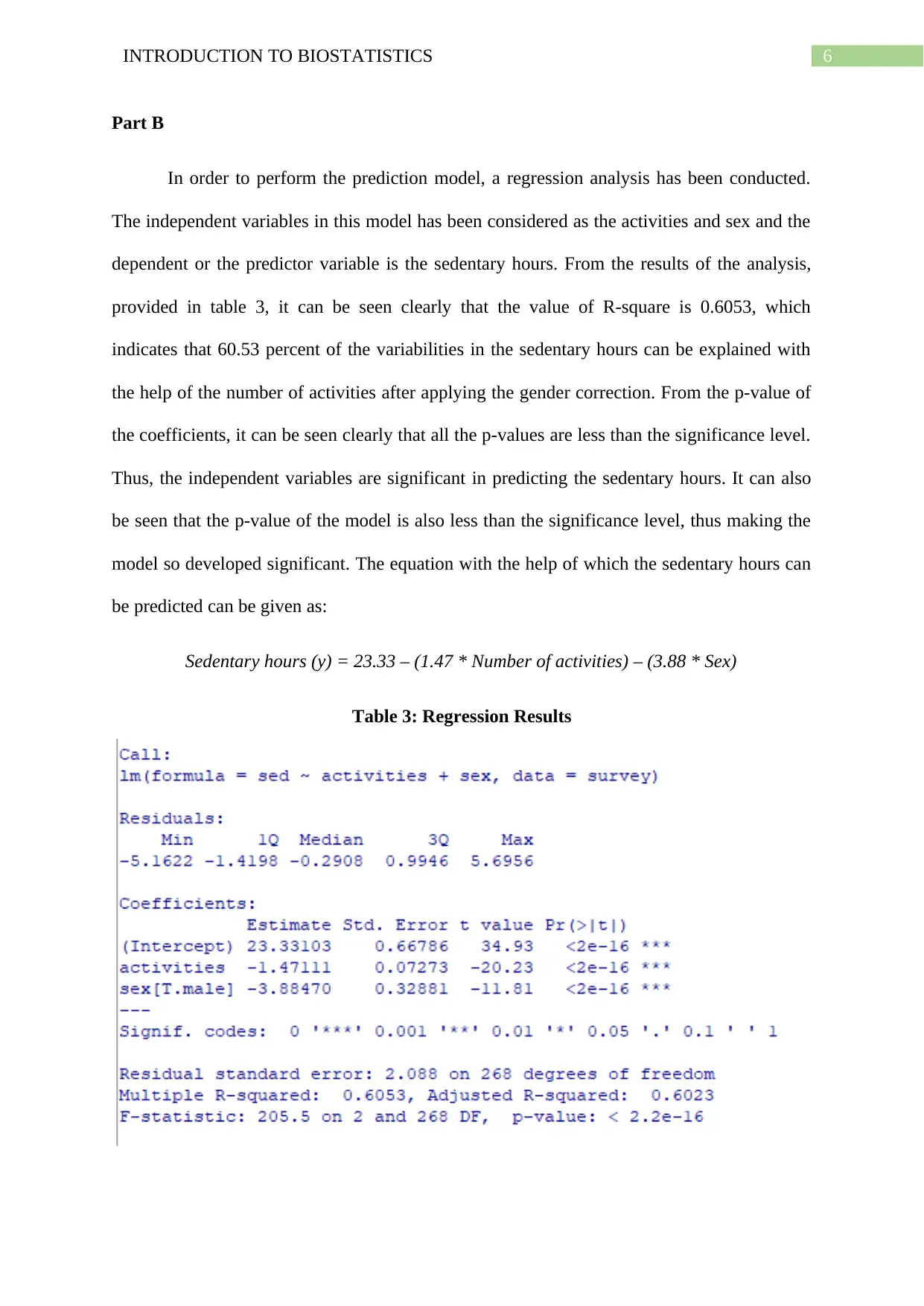
This biostatistics assignment comprises two main parts. The first part involves a critical evaluation of the article "Transport behaviours among older teenagers from semi-rural New Zealand" by Ward et al. (2015), focusing on the study's methodology and adherence to the STROBE checklist items 10, 12-17, highlighting issues such as sample size determination, data presentation, and the handling of missing data. The second part presents a statistical analysis, including descriptive statistics (frequency tables, pie charts, histograms) of gender, activities, and sedentary hours, followed by a regression analysis to predict sedentary hours based on the number of activities and gender. The analysis reveals that the number of activities has a significant impact on predicting sedentary hours after applying gender correction, with an R-square value of 0.6053, indicating that 60.53% of the variability in sedentary hours can be explained by the model.

Running Head: INTRODUCTION TO BIOSTATISTICS
Introduction to Biostatistics
Name of the Student
Name of the University
Student ID

1INTRODUCTION TO BIOSTATISTICS
Answer 1
In this part of the assignment, a critical evaluation of the article “Transport behaviours
among older teenagers from semi-rural New Zealand” written by Ward et al. (2015) will be
done based on the checklist provided by Strobe, on the items 10, 12 – 17.
Item 10:
The design of the determination of sample size is not proper in the article. The
number of participating schools have been mentioned in the article, which is 12. Out the 12
participating secondary schools, out of which 8 schools conducted the survey in class and the
rest of the 4 schools conducted the survey at home. There is only mention of the total number
of participating students in the survey, but the number of participating students in class and at
home is not mentioned in the article. Further, there is classification of gender among the
participants and the total number of male and female students have been mentioned, but the
number of male and female students with their preferring mode of transport has not been
mentioned.
Item 12:
The preference of the students on the mode of transport has been mentioned in the
article in frequencies as well as in percentages of the total number of participants. The
transport frustration over the last month has also been mentioned in frequencies as well as in
percentages. But the classification is only performed on the total number of participants and
not on the total number of participants from each gender. There is no mention of missing
dada and how it has been controlled in the whole analysis. There has been no explanation of
the chi square test in the article as well.

2INTRODUCTION TO BIOSTATISTICS
Item 13:
There is only mention of the response rates of the participants from the selected 12
secondary schools as well as the response rates of the students responding the survey in class
and at home. There has been no mention of the total number of students, the total number of
students at home as well as in class anywhere in the whole article.
Item 14:
The demographic profile of the students participating in the survey has been analysed
in the article. The age, gender, ethnicity, residing area and weekly income has been analysed.
No discussion about the missing data has been there in the article.
Item 15:
The article sheds light on the summary measures of the students, which is provided in
table 3 in the article. Only the mean and the standard deviation along with the maximum and
minimum numbers of activities and sedentary hours has been provided. This has been
classified according to the total number of students, male students and female students.
Item 16:
The analysis of the variables has been performed using chi-square test. Only the
significance of the tests has been discussed but no information about the confidence interval
has been discussed.
Item 17:
In this paper, the association between the different subgroups has been provided, but
no discussion about the sensitivity of the results has been discussed.

3INTRODUCTION TO BIOSTATISTICS
Answer 2
Part A
The 17-year residents of New South Wales in the selected 12 schools. This research
has been conducted to predict the sedentary hours each week with the help of the number of
activities by correcting gender. Before conducting the analysis, summary of the variables
involved in the analysis has been conducted. The summary of the variables is presented in
tables 1 and 2 and are illustrated with the help of pie charts and histograms in figures 1, 2 and
3 respectively.
Table 1: Frequency table for Gender
Gender Count Percentage
Male 141 52.03
Female 130 47.47
Figure 1: Pie Chart showing the proportion of Male and Female

4INTRODUCTION TO BIOSTATISTICS
Table 2: Summary Table for Number of Activities and Sedentary Hours
Statistics Activities Sed
Mean 7.336 10.518
Standard Deviation 2.263 3.311
Standard Error of Mean 0.137 0.201
Inter Quartile Range 3.0 4.5
Coefficient of Variation 0.308 0.315
Skewness 0.020 0.615
Kurtosis -0.424 -0.416
Minimum 1 4.1
Maximum 12 20.2
Quartiles
25% 6.0 8.2
50% 7.0 9.9
75% 9.0 12.7
Count 271 271

5INTRODUCTION TO BIOSTATISTICS
Figure 2: Histogram showing the Number of activities in the last month
Figure 3: Histogram showing the Sedentary Hours each Week

6INTRODUCTION TO BIOSTATISTICS
Part B
In order to perform the prediction model, a regression analysis has been conducted.
The independent variables in this model has been considered as the activities and sex and the
dependent or the predictor variable is the sedentary hours. From the results of the analysis,
provided in table 3, it can be seen clearly that the value of R-square is 0.6053, which
indicates that 60.53 percent of the variabilities in the sedentary hours can be explained with
the help of the number of activities after applying the gender correction. From the p-value of
the coefficients, it can be seen clearly that all the p-values are less than the significance level.
Thus, the independent variables are significant in predicting the sedentary hours. It can also
be seen that the p-value of the model is also less than the significance level, thus making the
model so developed significant. The equation with the help of which the sedentary hours can
be predicted can be given as:
Sedentary hours (y) = 23.33 – (1.47 * Number of activities) – (3.88 * Sex)
Table 3: Regression Results